suppressPackageStartupMessages({
  library(IsoformSwitchAnalyzeR)
  library(rtracklayer)
  library(ggrepel)
  library(scales)
  library(GenomicFeatures)
  library(DescTools)
  library(tidyverse)
  library(magrittr)
})

colorVector = c(
  "Known" = "#009E73",
  "ISM"   = "#0072B2",
  "ISM_Prefix" = "#005996",
  "ISM_Suffix" = "#378bcc",
  "NIC"   = "#D55E00",
  "NNC"   = "#E69F00",
  "Other" = "#000000"
)
colorVector_ismSplit = colorVector[-2]Figure 1 - BulkTxomeAnalysis
Load Data
if(!file.exists("data/working/bulkTxome.Rdata")) {
  talon_gtf = rtracklayer::import("data/cp_vz_0.75_min_7_recovery_talon.gtf.gz")
  tx.isoseq =  talon_gtf %>% as_tibble() %>% filter(type == "transcript")

  sqanti_gtf = rtracklayer::import("data/sqanti/cp_vz_0.75_min_7_recovery_talon_corrected.gtf.cds.gtf.gz")
  tx.sqanti = sqanti_gtf %>% as_tibble() %>% filter(type == "transcript")

  gencode_gtf = rtracklayer::import("ref/gencode.v33lift37.annotation.gtf.gz")
  tx.gencode =  gencode_gtf %>% as_tibble() %>% filter(type == "transcript")

  txdb.gencode = makeTxDbFromGRanges(gencode_gtf)
  gencodelengths= transcriptLengths(txdb.gencode)

  txdb.isoseq = makeTxDbFromGRanges(talon_gtf)
  isoSeqLengths = transcriptLengths(txdb.isoseq)
  samps = tribble(
    ~sample_id, ~condition,
    "VZ_209", "VZ",
    "VZ_334", "VZ",
    "VZ_336", "VZ",
    "CP_209", "CP",
    "CP_334", "CP",
    "CP_336", "CP"
  ) %>%
    dplyr::mutate(
      dplyr::across(condition, as_factor)
    )

  cts = read_table("data/cp_vz_0.75_min_7_recovery_talon_abundance_filtered.tsv.gz")
  cts.collapse = cts %>%
    mutate(
      VZ_209 = rowSums(across(matches("209_.*_VZ"))),
      VZ_334 = rowSums(across(matches("334_.*_VZ"))),
      VZ_336 = rowSums(across(matches("336_.*_VZ"))),
      CP_209 = rowSums(across(matches("209_.*_CP"))),
      CP_334 = rowSums(across(matches("334_.*_CP"))),
      CP_336 = rowSums(across(matches("336_.*_CP"))),
      .keep = "unused"
    ) %>%
    dplyr::select(!c("gene_ID", "transcript_ID", "annot_transcript_name")) %>%
    dplyr::rename(
      gene_id = "annot_gene_id",
      transcript_id = "annot_transcript_id",
      gene_name = "annot_gene_name"
    ) %>%
    mutate(
      gene_novelty = as.factor(gene_novelty),
      transcript_novelty = as.factor(transcript_novelty),
      ISM_subtype = ISM_subtype %>% na_if("None") %>% as.factor()
    )
  cts$counts = rowSums(as.matrix(cts.collapse[,9:14]))

  cts$novelty2 = as.character(cts$transcript_novelty)
  cts$novelty2[which(cts$novelty2=="ISM" & cts$ISM_subtype=="Prefix")] = "ISM_Prefix"
  cts$novelty2[which(cts$novelty2=="ISM" & cts$ISM_subtype=="Suffix")] = "ISM_Suffix"
  cts$novelty2[cts$novelty2 %in% c("Antisense", "Genomic", "Intergenic", "ISM")] = "Other"
  cts$novelty2 = factor(cts$novelty2,levels=c("Known", "ISM_Prefix", "ISM_Suffix", "NIC", "NNC", "Other"))


  TableS1 = tx.isoseq %>% dplyr::select(gene_id, transcript_id, gene_name, transcript_name, seqnames, start, end, strand, transcript_length=width, source, gene_status, gene_type, transcript_status,transcript_type,  havana_transcript, ccdsid, protein_id)
  TableS1 = TableS1 %>% left_join(cts %>% dplyr::select(transcript_id=annot_transcript_id, transcript_novelty, ISM_subtype, transcript_novelty2 = novelty2, n_exons, cds_length = length, expression_counts = counts))
  TableS1$expression_TPM = TableS1$expression_counts / (sum(TableS1$expression_counts / 1000000))
  write_tsv(TableS1, file="output/tables/TableS1_transcript_annotation.tsv")
  save.image("data/working/bulkTxome.Rdata")
} else {
  load("data/working/bulkTxome.Rdata")
}
Warning in .get_cds_IDX(mcols0$type, mcols0$phase): The "phase" metadata column contains non-NA values for features of type
stop_codon. This information was ignored.Warning in .reject_transcripts(bad_tx, because): The following transcripts were dropped because they have incompatible
CDS and stop codons: ENST00000422803.2_2, ENST00000618549.1_2,
ENST00000619291.4_2, ENST00000621077.1_2, ENST00000621229.1_2,
ENST00000631326.2_2
── Column specification ────────────────────────────────────────────────────────
cols(
  .default = col_double(),
  annot_gene_id = col_character(),
  annot_transcript_id = col_character(),
  annot_gene_name = col_character(),
  annot_transcript_name = col_character(),
  gene_novelty = col_character(),
  transcript_novelty = col_character(),
  ISM_subtype = col_character()
)
ℹ Use `spec()` for the full column specifications.
Joining, by = "transcript_id"Technical and Biological Replicates
Fig1B: Isoform level MDS
##
length(unique(cts$annot_transcript_id)) #214516 total isoforms
[1] 214516length(unique(cts$annot_gene_id)) #24554 genes[1] 24554## Collapsing across technical replicates
countMat = as.matrix(cts.collapse[,9:14])
cs = colSums(countMat) / 1000000 ## TPM normalize
countMat.tpm = t(apply(countMat, 1, function(x) { x / cs}))
table(rowSums(countMat.tpm > 0.1) >3) ## 175730 isoforms @ TPM > 0.1 in half of samples
 FALSE   TRUE
38786 175730 table(rowSums(countMat.tpm > 1) >3) ## 58102 @ TPM > 1 in half of samples
 FALSE   TRUE
156414  58102
expressedIsoforms = rowSums(countMat.tpm > .1) >3 ## TPM > .1 in half of samples
length(unique(cts$annot_gene_id[expressedIsoforms])) ## 17,299 genes with expressed isoforms (TPM > .1)[1] 17299# Analyze technical replicates separately
cts.all = cts[,12:35]
cs = colSums(cts.all) / 1000000
cts.all.tpm = t(apply(cts.all, 1, function(x) { x / cs}))
mds = cmdscale(dist(t(log2(.1+cts.all.tpm))),k = 4)
df = data.frame(sample=rownames(mds), PC1 = mds[,1], PC2=mds[,2], PC3=mds[,3], PC4=mds[,4])
df$Region = substr(df$sample, 7,9)
df$Subject = substr(df$sample, 1,3)
df$batch = substr(df$sample, 5,5)
Fig1B=ggplot(df, aes(x=PC1,y=PC2, color=Region, shape=Subject,label=batch)) + geom_point(size=4) + geom_text(color='black', size=2) + theme_bw() + ggtitle("Isoform level clustering")
Fig1B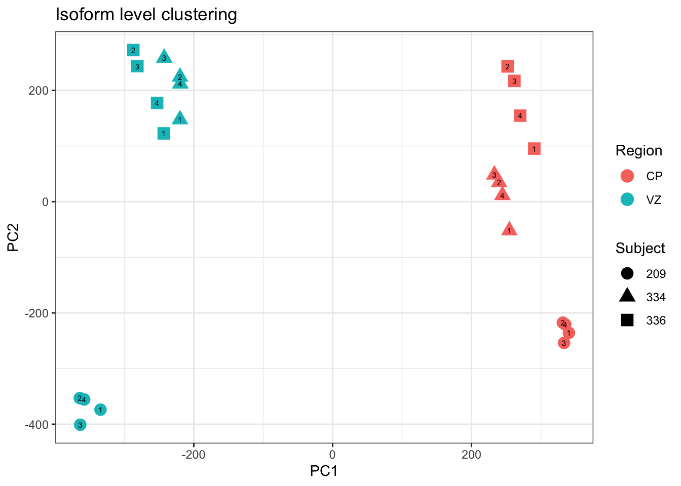
ggsave(Fig1B,filename = "output/figures/Fig1/Fig1B.pdf", width = 3.5,height=2)Fig1C: smoothscatter
geneCountMap.tpm = tibble(gene = cts$annot_gene_name, as_tibble(cts.all.tpm)) %>% group_by(gene) %>%  summarise(across(everything(), sum))
mds = cmdscale(dist(t(log2(.1+geneCountMap.tpm %>% dplyr::select(-gene)))),k = 4)
df = data.frame(sample=rownames(mds), PC1 = mds[,1], PC2=mds[,2], PC3=mds[,3], PC4=mds[,4])
df$Region = substr(df$sample, 7,9)
df$Subject = substr(df$sample, 1,3)
df$TechnicalReplicate = substr(df$sample, 5,5)
#ggplot(df, aes(x=PC1,y=PC2, color=Region, shape=Subject)) + geom_point(size=3) + theme_bw() + ggtitle("Gene level clustering")

Fig1C=ggplot(as.data.frame(countMat.tpm), aes(x=log2(1+VZ_334), y=log2(1+VZ_336))) + geom_point(color='blue',size=.4,alpha=.5) + theme_bw() + geom_abline(slope=1,lty=2) + geom_smooth(method='lm',color='black') + ggtitle("R=0.93, p<2e-16")
Fig1C
`geom_smooth()` using formula 'y ~ x'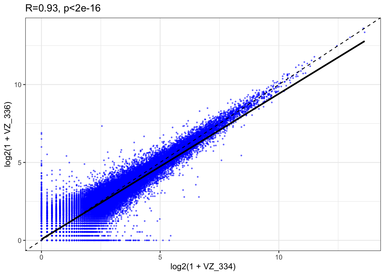
ggsave(Fig1C ,filename = "output/figures/Fig1/Fig1C.pdf", width = 3,height=3)`geom_smooth()` using formula 'y ~ x'pdf(file= "output/figures/Fig1/Fig1Cb.pdf", width = 4, height=4)
smoothScatter(log2(1+countMat.tpm[,"VZ_334"]), log2(1+countMat.tpm[,"VZ_336"]))
dev.off()quartz_off_screen
2 smoothScatter(log2(1+countMat.tpm[,"VZ_334"]), log2(1+countMat.tpm[,"VZ_336"]))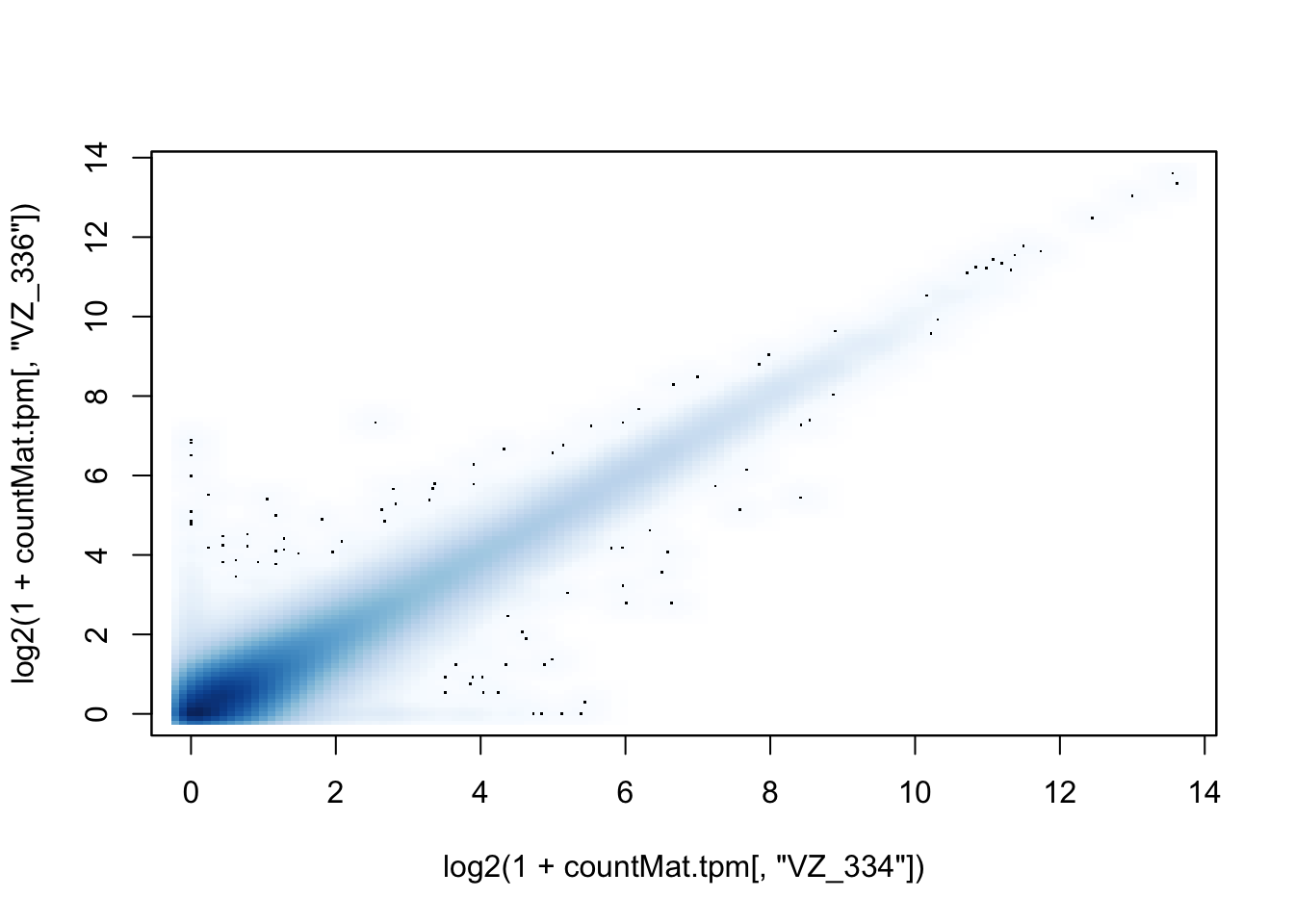
panel.cor <- function(x, y, digits = 2, prefix = "R=", cex.cor, ...)
{
    usr <- par("usr"); on.exit(par(usr))
    par(usr = c(0, 1, 0, 1))
    r <- abs(cor(x, y))
    txt <- format(c(r, 0.123456789), digits = digits)[1]
    txt <- paste0(prefix, txt)
    if(missing(cex.cor)) cex.cor <- 0.8/strwidth(txt)
    text(0.5, 0.5, txt, cex =1)
}

pdf(file="output/figures/supplement/FigS2_bio_replicates.pdf", width=8,height=6)
pairs(log2(1+countMat.tpm), panel=function(x,y){smoothScatter(x,y,add=T)},upper.panel = panel.cor)
dev.off()
quartz_off_screen
2 Fig1E: tx novelty
Fig1E = ggplot(cts %>% filter(counts>10,), aes(x=counts, fill=novelty2)) + geom_histogram(position=position_fill(),alpha=.75, binwidth = .3)+ theme_bw()  +  scale_x_log10()+
  annotation_logticks(scaled = T,sides='b')+ theme(panel.grid.minor = element_blank()) + labs(x="Min observed counts", y="Proportion of transcripts") + ggtitle("Transcript novelty & type") + theme(plot.title = element_text(hjust=.5))  + scale_fill_manual(values=colorVector_ismSplit)
Fig1E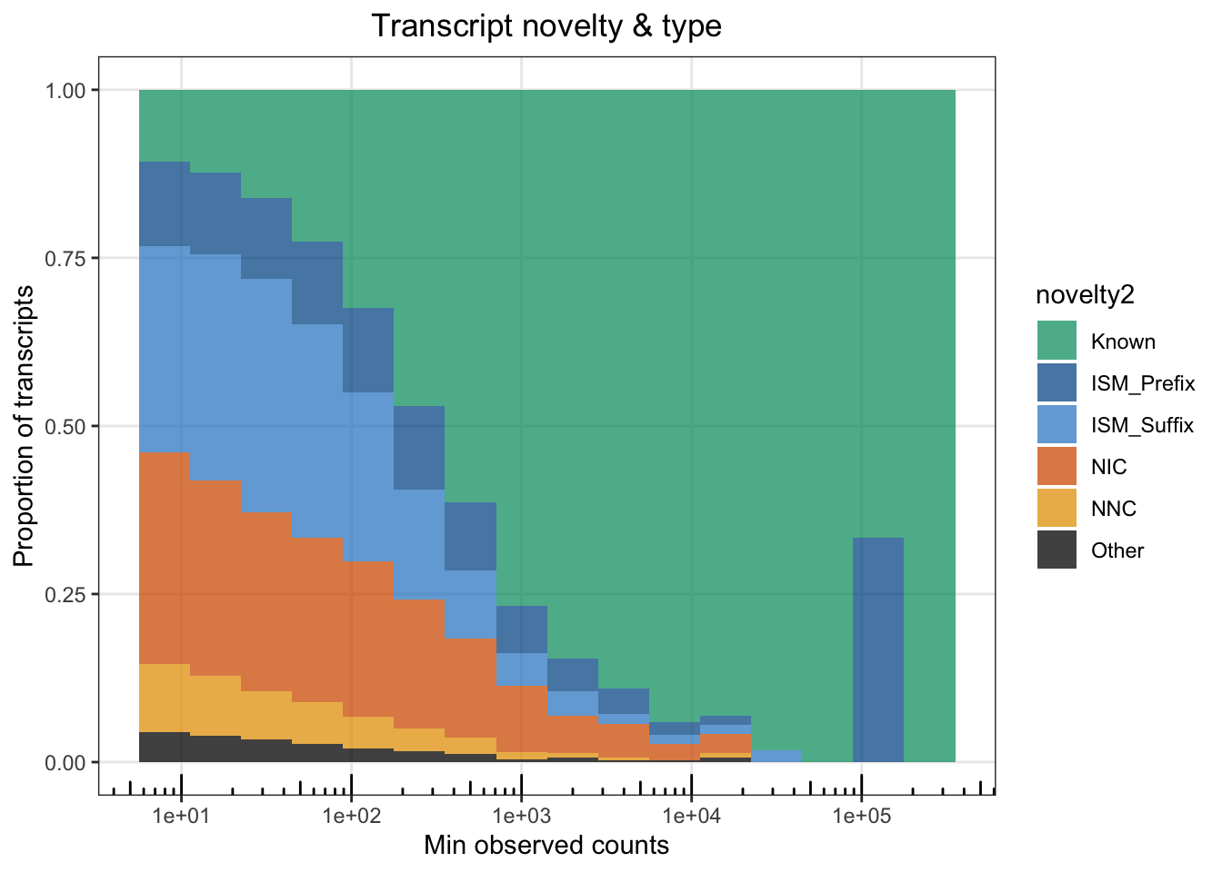
ggsave(file="output/figures/Fig1/Fig1E.pdf",width=5,height=3)

## Removing MAP1B
ggplot(cts %>% filter(counts>10,annot_gene_name!="MAP1B"), aes(x=counts, fill=novelty2)) + geom_histogram(position=position_fill(),alpha=.5, binwidth = .3)+ theme_bw()  +  scale_x_log10()+
  annotation_logticks(scaled = T,sides='b')+ theme(panel.grid.minor = element_blank()) + labs(x="Min observed counts", y="Proportion of transcripts") + ggtitle("Transcript novelty & type",subtitle = '(MAP1B removed)') + theme(plot.title = element_text(hjust=.5))  + scale_fill_manual(values=colorVector_ismSplit)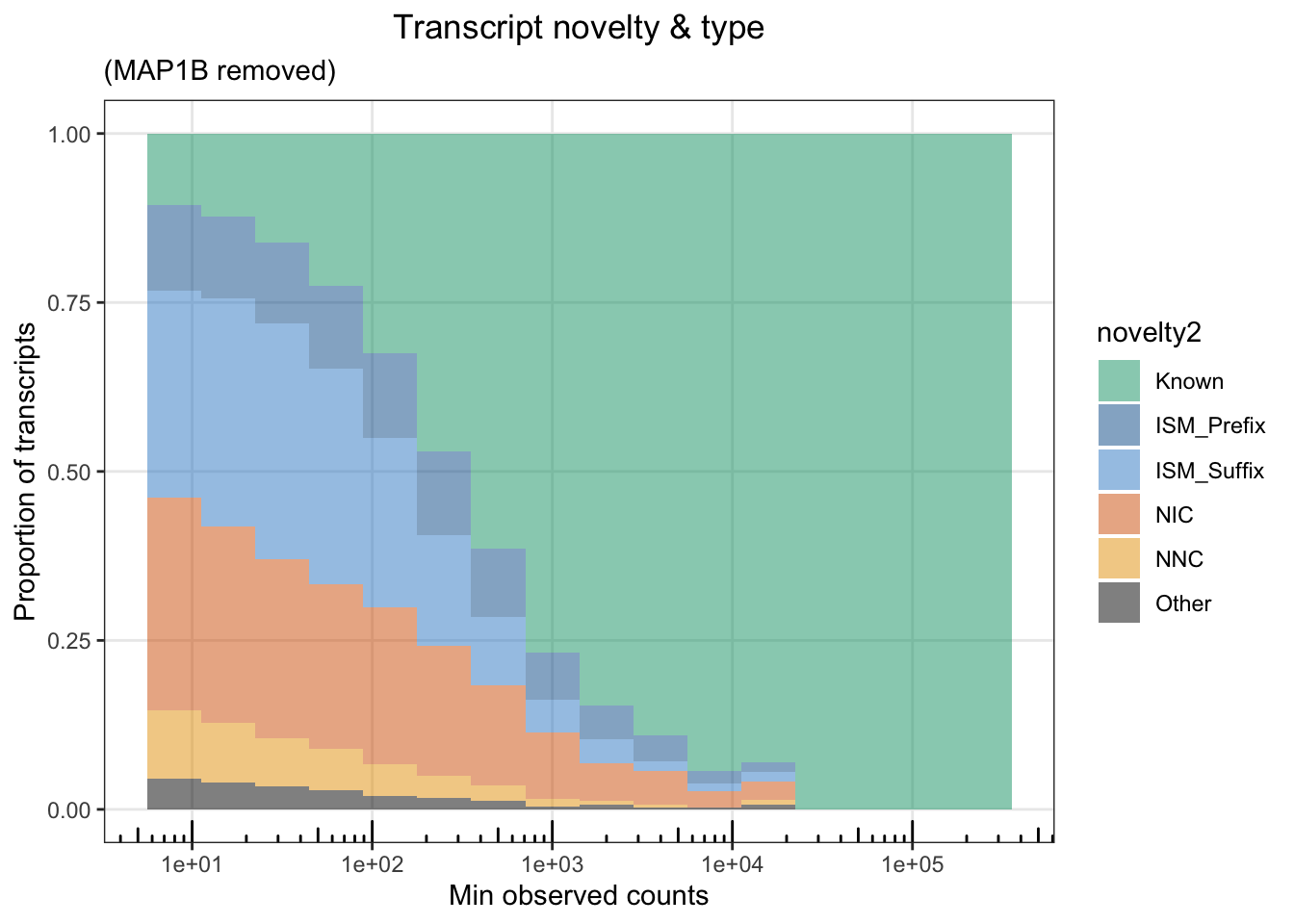
Analyses of Transcript Length
Fig1F: Tx Length Histogra
df<- cts%>% dplyr::select("annot_transcript_id", "transcript_novelty", "ISM_subtype", "annot_gene_name", "counts") %>% right_join(isoSeqLengths, by=c("annot_transcript_id" = "tx_name"))

df$novelty2 = as.character(df$transcript_novelty)
df$novelty2[which(df$novelty2=="ISM" & df$ISM_subtype=="Prefix")] = "ISM_Prefix"
df$novelty2[which(df$novelty2=="ISM" & df$ISM_subtype=="Suffix")] = "ISM_Suffix"
df$novelty2[df$novelty2 %in% c("Antisense", "Genomic", "Intergenic", "ISM")] = "Other"
df$novelty2 = factor(df$novelty2,levels=c("Known", "ISM_Prefix", "ISM_Suffix", "NIC", "NNC", "Other"))

df %>% filter(tx_len > 900, tx_len < 6000) %>% group_by(novelty2) %>% summarise(peak=10^mean(log10(tx_len)), median(tx_len), mean(tx_len))
# A tibble: 6 × 4
novelty2 peak `median(tx_len)` `mean(tx_len)`
<fct> <dbl> <dbl> <dbl>
1 Known 2305. 2317 2588.
2 ISM_Prefix 2604. 2701 2809.
3 ISM_Suffix 2833. 2914 3019.
4 NIC 3023. 3100 3193.
5 NNC 2867. 2953 3033.
6 Other 2616. 2716 2807.Fig1F = ggplot(df, aes(x=tx_len, fill=novelty2)) + geom_histogram(alpha=.75,binwidth = .03)+
theme_bw() + scale_fill_manual(values=colorVector_ismSplit) +
scale_x_continuous(trans = log10_trans(),breaks = trans_breaks("log10", function(x) 10^x),
labels = trans_format("log10", math_format(10^.x)),limits = c(50,10^5)) + annotation_logticks() +
labs(x="Transcript Length (bp)") + ggtitle("Transcript length distribution")
Fig1FWarning: Removed 6 rows containing non-finite values (stat_bin).Warning: Removed 12 rows containing missing values (geom_bar).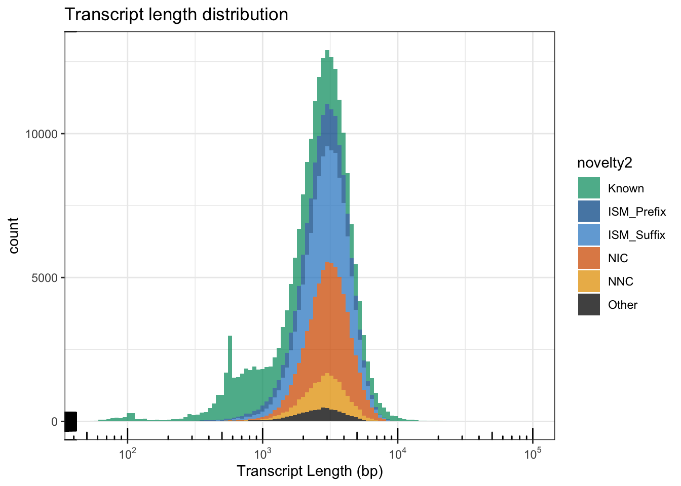
ggsave(Fig1F,file='output/figures/Fig1/Fig1F.pdf', width=5,height=2.5)Warning: Removed 6 rows containing non-finite values (stat_bin).
Removed 12 rows containing missing values (geom_bar).## Zoomed in
ggplot(df, aes(x=tx_len, fill=novelty2)) + geom_histogram(alpha=.5,binwidth = 100)+
theme_bw() + scale_fill_manual(values=colorVector_ismSplit) + xlim(800,5500) +
labs(x="Transcript Length (bp)") + ggtitle("Transcript length distribution") +
geom_vline(xintercept = 2588, lty=2,color="#009E73")Warning: Removed 27594 rows containing non-finite values (stat_bin).
Removed 12 rows containing missing values (geom_bar).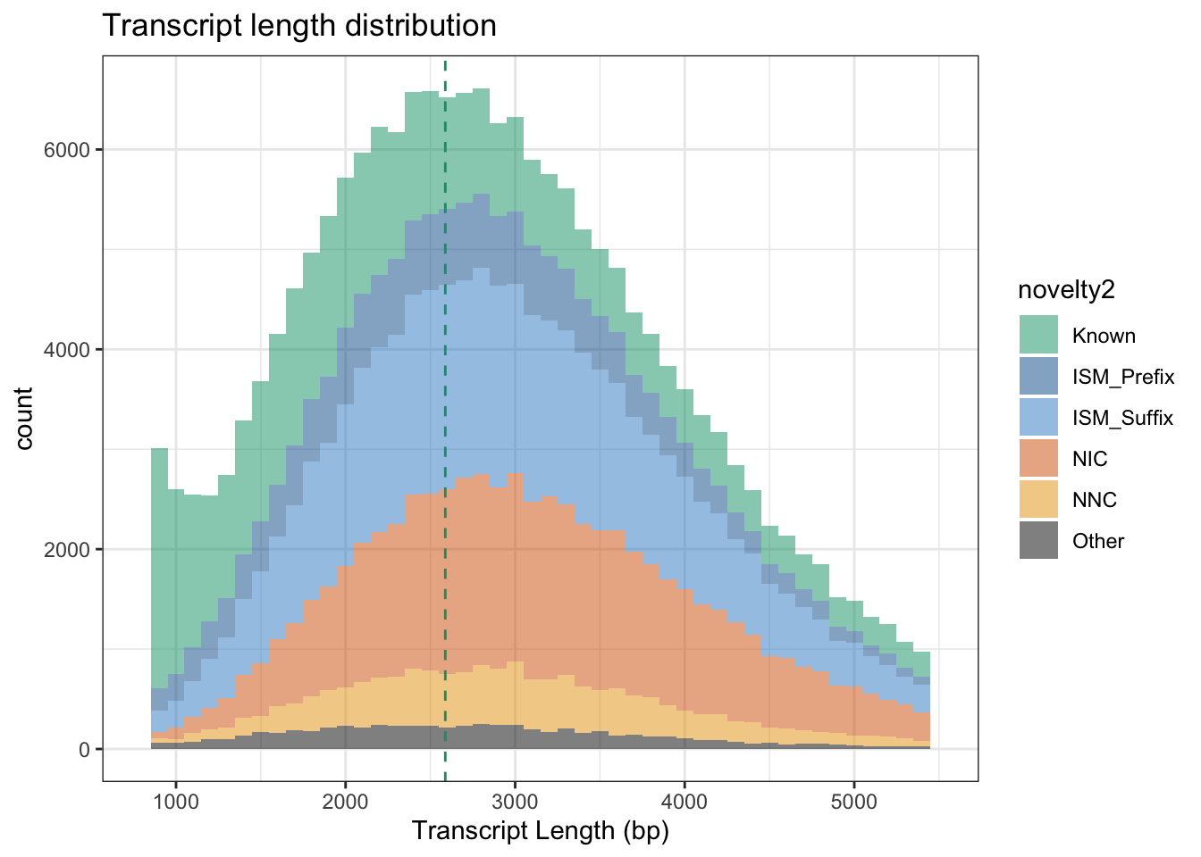
mean(df$tx_len[df$novelty2=="Known"])[1] 2276.283sd(df$tx_len[df$novelty2=="Known"])[1] 2224.66mean(df$tx_len[df$novelty2!="Known"])[1] 3072.309sd(df$tx_len[df$novelty2!="Known"])[1] 1168.997## Linear model: Known is the intercept
summary(lm(log2(tx_len) ~ novelty2,data=df[df$tx_len > 1000,]))
Call:
lm(formula = log2(tx_len) ~ novelty2, data = df[df$tx_len > 1000,
    ])

Residuals:
    Min      1Q  Median      3Q     Max
-1.6246 -0.3952  0.0137  0.3949  6.2778

Coefficients:
                    Estimate Std. Error  t value Pr(>|t|)
(Intercept)        11.367558   0.002874 3955.796  < 2e-16 ***
novelty2ISM_Prefix  0.016804   0.005031    3.341 0.000836 ***
novelty2ISM_Suffix  0.126745   0.003850   32.923  < 2e-16 ***
novelty2NIC         0.224224   0.003922   57.172  < 2e-16 ***
novelty2NNC         0.137284   0.005755   23.855  < 2e-16 ***
novelty2Other       0.012843   0.008076    1.590 0.111768
---
Signif. codes:  0 '***' 0.001 '**' 0.01 '*' 0.05 '.' 0.1 ' ' 1

Residual standard error: 0.5991 on 190337 degrees of freedom
Multiple R-squared:  0.0208,    Adjusted R-squared:  0.02078
F-statistic: 808.7 on 5 and 190337 DF, p-value: < 2.2e-16summary(lm(log2(tx_len) ~ novelty2=="Known",data=df))
Call:
lm(formula = log2(tx_len) ~ novelty2 == "Known", data = df)

Residuals:
    Min      1Q  Median      3Q     Max
-5.5655 -0.4458  0.0731  0.5117  7.0423

Coefficients:
                         Estimate Std. Error t value Pr(>|t|)
(Intercept)             11.472348   0.002319  4948.1   <2e-16 ***
novelty2 == "Known"TRUE -0.869348   0.004212  -206.4   <2e-16 ***
---
Signif. codes:  0 '***' 0.001 '**' 0.01 '*' 0.05 '.' 0.1 ' ' 1

Residual standard error: 0.8965 on 214514 degrees of freedom
Multiple R-squared:  0.1657,    Adjusted R-squared:  0.1657
F-statistic: 4.26e+04 on 1 and 214514 DF,  p-value: < 2.2e-16
## Non-parametric test
kruskal.test((tx_len) ~ novelty2=="Known",data=df)
    Kruskal-Wallis rank sum test

data:  (tx_len) by novelty2 == "Known"
Kruskal-Wallis chi-squared = 23404, df = 1, p-value < 2.2e-16kruskal.test(log2(tx_len) ~ novelty2,data=df[df$tx_len > 1000,])
    Kruskal-Wallis rank sum test

data:  log2(tx_len) by novelty2
Kruskal-Wallis chi-squared = 4511.4, df = 5, p-value < 2.2e-16DescTools::DunnTest(log2(tx_len) ~ novelty2, data=df[df$tx_len > 1000,], method='bonferroni')
 Dunn's test of multiple comparisons using rank sums : bonferroni

                      mean.rank.diff    pval
ISM_Prefix-Known           3089.5845 3.2e-10 ***
ISM_Suffix-Known          13024.1853 < 2e-16 ***
NIC-Known                 22131.1682 < 2e-16 ***
NNC-Known                 13892.0679 < 2e-16 ***
Other-Known                2480.9445  0.0121 *
ISM_Suffix-ISM_Prefix      9934.6008 < 2e-16 ***
NIC-ISM_Prefix            19041.5837 < 2e-16 ***
NNC-ISM_Prefix            10802.4834 < 2e-16 ***
Other-ISM_Prefix           -608.6399  1.0000
NIC-ISM_Suffix             9106.9829 < 2e-16 ***
NNC-ISM_Suffix              867.8826  1.0000
Other-ISM_Suffix         -10543.2407 < 2e-16 ***
NNC-NIC                   -8239.1003 < 2e-16 ***
Other-NIC                -19650.2236 < 2e-16 ***
Other-NNC                -11411.1233 < 2e-16 ***
---
Signif. codes:  0 '***' 0.001 '**' 0.01 '*' 0.05 '.' 0.1 ' ' 1
## Boxplot
# ggplot(df, aes(x=novelty2, y=tx_len, fill=novelty2)) + geom_boxplot()+
# theme_bw() + scale_fill_manual(values=colorVector_ismSplit) +
# scale_y_continuous(trans = log10_trans(),breaks = trans_breaks("log10", function(x) 10^x),
# labels = trans_format("log10", math_format(10^.x)))Fig1G: # Exons / gene
Fig1G = ggplot(df, aes(x=nexon, fill=novelty2)) + geom_histogram(alpha=.75, binwidth = 1) + theme_bw() +
  xlim(1,40) + scale_fill_manual(values=colorVector_ismSplit) + labs(x="# Exons", y="# Transcripts") + ggtitle('Exons per  Transcript') + theme(legend.position = "none")
Fig1G
Warning: Removed 597 rows containing non-finite values (stat_bin).Warning: Removed 12 rows containing missing values (geom_bar).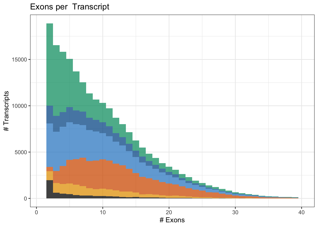
ggsave(Fig1G,file='output/figures/Fig1/Fig1G.pdf', width=3,height=2.5)Warning: Removed 597 rows containing non-finite values (stat_bin).
Removed 12 rows containing missing values (geom_bar).df %>% group_by(novelty2) %>% dplyr::select(nexon) %>% summarise(median(nexon), mean(nexon), sd(nexon), quantile(nexon, .05), quantile(nexon,.95))Adding missing grouping variables: `novelty2`# A tibble: 6 × 6
novelty2 `median(nexon)` `mean(nexon)` `sd(nexon)` quantile(nexon,…¹ quant…²
<fct> <dbl> <dbl> <dbl> <dbl> <dbl>
1 Known 5 7.16 6.88 1 21
2 ISM_Prefix 8 10.1 6.99 2 23
3 ISM_Suffix 8 10.1 7.01 2 24
4 NIC 12 13.2 7.31 4 27
5 NNC 9 10.3 6.80 2 23
6 Other 5 7.30 6.24 2 20
# … with abbreviated variable names ¹`quantile(nexon, 0.05)`,
# ²`quantile(nexon, 0.95)`df %>% group_by(novelty2=="Known") %>% dplyr::select(nexon) %>% summarise(median(nexon), mean(nexon), sd(nexon), quantile(nexon, .05), quantile(nexon,.95))Adding missing grouping variables: `novelty2 == "Known"`# A tibble: 2 × 6
`novelty2 == "Known"` `median(nexon)` `mean(nexon)` sd(nexon…¹ quant…² quant…³
<lgl> <dbl> <dbl> <dbl> <dbl> <dbl>
1 FALSE 10 11.0 7.25 2 25
2 TRUE 5 7.16 6.88 1 21
# … with abbreviated variable names ¹`sd(nexon)`, ²`quantile(nexon, 0.05)`,
# ³`quantile(nexon, 0.95)`# Linear model (known is intercept)
summary(lm(log2(df$nexon) ~ df$novelty2))
Call:
lm(formula = log2(df$nexon) ~ df$novelty2)

Residuals:
    Min      1Q  Median      3Q     Max
-2.4927 -0.6853  0.0657  0.8222  4.0657

Coefficients:
                      Estimate Std. Error t value Pr(>|t|)
(Intercept)           2.256270   0.004331 520.977   <2e-16 ***
df$novelty2ISM_Prefix 0.720984   0.008605  83.788   <2e-16 ***
df$novelty2ISM_Suffix 0.728883   0.006378 114.275   <2e-16 ***
df$novelty2NIC        1.236409   0.006545 188.897   <2e-16 ***
df$novelty2NNC        0.776082   0.010123  76.663   <2e-16 ***
df$novelty2Other      0.127124   0.014200   8.952   <2e-16 ***
---
Signif. codes:  0 '***' 0.001 '**' 0.01 '*' 0.05 '.' 0.1 ' ' 1

Residual standard error: 1.104 on 214510 degrees of freedom
Multiple R-squared:  0.1525,    Adjusted R-squared:  0.1525
F-statistic:  7720 on 5 and 214510 DF,  p-value: < 2.2e-16
## Non-parametric test
kruskal.test(log2(df$nexon) ~ as.factor(df$novelty2))
    Kruskal-Wallis rank sum test

data:  log2(df$nexon) by as.factor(df$novelty2)
Kruskal-Wallis chi-squared = 29541, df = 5, p-value < 2.2e-16kruskal.test(log2(df$nexon) ~ as.factor(df$novelty2=="Known"))
    Kruskal-Wallis rank sum test

data:  log2(df$nexon) by as.factor(df$novelty2 == "Known")
Kruskal-Wallis chi-squared = 20319, df = 1, p-value < 2.2e-16kruskal.test((df$nexon) ~ as.factor(df$novelty2=="Known"))
    Kruskal-Wallis rank sum test

data:  (df$nexon) by as.factor(df$novelty2 == "Known")
Kruskal-Wallis chi-squared = 20319, df = 1, p-value < 2.2e-16DescTools::DunnTest(log2(df$nexon) ~ as.factor(df$novelty2),method='bonferroni')
 Dunn's test of multiple comparisons using rank sums : bonferroni

                      mean.rank.diff    pval
ISM_Prefix-Known          32693.6946 < 2e-16 ***
ISM_Suffix-Known          33127.7388 < 2e-16 ***
NIC-Known                 61043.3188 < 2e-16 ***
NNC-Known                 35434.2011 < 2e-16 ***
Other-Known                3206.1675 0.00083 ***
ISM_Suffix-ISM_Prefix       434.0442 1.00000
NIC-ISM_Prefix            28349.6241 < 2e-16 ***
NNC-ISM_Prefix             2740.5065 0.00050 ***
Other-ISM_Prefix         -29487.5271 < 2e-16 ***
NIC-ISM_Suffix            27915.5799 < 2e-16 ***
NNC-ISM_Suffix             2306.4623 0.00092 ***
Other-ISM_Suffix         -29921.5713 < 2e-16 ***
NNC-NIC                  -25609.1177 < 2e-16 ***
Other-NIC                -57837.1512 < 2e-16 ***
Other-NNC                -32228.0336 < 2e-16 ***
---
Signif. codes:  0 '***' 0.001 '**' 0.01 '*' 0.05 '.' 0.1 ' ' 1
Analyses of transcripts per gene & disease
NDD risk genes ~ unique transcipts per gene
source("code/risk_genes.R")Warning: One or more parsing issues, see `problems()` for detailsRows: 18321 Columns: 26
── Column specification ────────────────────────────────────────────────────────
Delimiter: "\t"
chr (8): gene_id, group, OR (PTV), OR (Class I), OR (Class II), OR (PTV) up...
dbl (16): Case PTV, Ctrl PTV, Case mis3, Ctrl mis3, Case mis2, Ctrl mis2, P ...
lgl (2): De novo mis3, De novo mis2
ℹ Use `spec()` to retrieve the full column specification for this data.
ℹ Specify the column types or set `show_col_types = FALSE` to quiet this message.
Rows: 119958 Columns: 20
── Column specification ────────────────────────────────────────────────────────
Delimiter: "\t"
chr (4): gene_id, group, damaging_missense_fisher_gnom_non_psych_OR, ptv_fi...
dbl (16): n_cases, n_controls, damaging_missense_case_count, damaging_missen...
ℹ Use `spec()` to retrieve the full column specification for this data.
ℹ Specify the column types or set `show_col_types = FALSE` to quiet this message.
Rows: 71456 Columns: 12
── Column specification ────────────────────────────────────────────────────────
Delimiter: "\t"
chr (2): gene_id, group
dbl (9): xcase_lof, xctrl_lof, pval_lof, xcase_mpc, xctrl_mpc, pval_mpc, xca...
lgl (1): pval_infrIndel
ℹ Use `spec()` to retrieve the full column specification for this data.
ℹ Specify the column types or set `show_col_types = FALSE` to quiet this message.risk_genes = read.csv("ref/ASD+SCZ+DDD_2022.csv")
pLI_scores = read.table('ref/pLI_scores.ensid.txt',header = T)
asd_genes = risk_genes$Gene[risk_genes$Set=="ASD (SFARI score 1)"]
ddd_genes = risk_genes$Gene[risk_genes$Set=="DDD (Kaplanis et al. 2019)"]
geneCounts = cts %>% group_by(gene_id=substr(annot_gene_id,1,15)) %>% summarise(gene_count = sum(counts))
geneCounts$gene_count = geneCounts$gene_count / (sum(geneCounts$gene_count) / 1000000)
talon_exons = talon_gtf[talon_gtf$type == "exon"]
#talon_exons_novel = talon_gtf[talon_gtf$type == "exon" & talon_gtf$transcript_status == "NOVEL"]
talon_exons_by_gene = split(talon_exons, talon_exons$gene_id)
#talon_exons_by_gene_novel = split(talon_exons_novel, talon_exons_novel$gene_id)
geneLengths = enframe(
sum(width(GenomicRanges::reduce(ranges(talon_exons_by_gene)))),
name = "gene_id",
value = "coding_length"
) %>%
left_join(
enframe(
max(end(talon_exons_by_gene)) - min(start(talon_exons_by_gene)) + 1,
name = "gene_id",
value = "talon_width" # due to novel/unexpressed transcripts, talon gene width can differ from gencode gene width
)
) %>%
# left_join(
# enframe(
# sum(width(GenomicRanges::reduce(ranges(talon_exons_by_gene_novel)))),
# name = "gene_id",
# value = "coding_length_novel"
# )
# ) %>%
mutate(gene_id = substr(gene_id, 1, 15))Joining, by = "gene_id"df <- talon_gtf %>% as_tibble() %>%
mutate(gene_id = str_sub(gene_id, 1, 15)) %>%
group_by(gene_id) %>%
summarize(n_transcripts = n_distinct(na.omit(transcript_id)), n_exons = n_distinct(na.omit(exon_id))) %>%
ungroup()
df <- as_tibble(gencode_gtf) %>% dplyr::filter(type=="gene") %>% mutate(gene_id=substr(gene_id,0,15)) %>% right_join(df, by="gene_id")
df <- df %>% left_join(geneCounts) Joining, by = "gene_id"df <- df %>% left_join(geneLengths)Joining, by = "gene_id"df <- pLI_scores %>% as_tibble() %>% dplyr::select(gene_id=gene, pLI) %>% right_join(df)Joining, by = "gene_id"df$gene_rank = rank(-df$n_transcripts, ties.method = 'first')
df$DDD = FALSE
df$DDD[df$gene_name %in% c(asd_genes, ddd_genes)] = TRUE
df = rareVar.binary %>% as_tibble(rownames = "gene_id") %>% right_join(df)Joining, by = "gene_id"s=summary(glm(NDD.fuTADA ~ log10(n_transcripts) + log10(width) + log10(gene_count) + log10(coding_length), data=df %>% filter(gene_type == "protein_coding"), family='binomial'))
print(s)
Call:
glm(formula = NDD.fuTADA ~ log10(n_transcripts) + log10(width) +
    log10(gene_count) + log10(coding_length), family = "binomial",
    data = df %>% filter(gene_type == "protein_coding"))

Deviance Residuals:
    Min       1Q   Median       3Q      Max
-1.1142  -0.3808  -0.2840  -0.1897   3.5966

Coefficients:
                      Estimate Std. Error z value Pr(>|z|)
(Intercept)          -11.13478    0.61994 -17.961  < 2e-16 ***
log10(n_transcripts)   0.44281    0.15209   2.912  0.00360 **
log10(width)           0.47907    0.08761   5.468 4.54e-08 ***
log10(gene_count)      0.21934    0.07888   2.781  0.00542 **
log10(coding_length)   1.39117    0.20486   6.791 1.11e-11 ***
---
Signif. codes:  0 '***' 0.001 '**' 0.01 '*' 0.05 '.' 0.1 ' ' 1

(Dispersion parameter for binomial family taken to be 1)

    Null deviance: 6026.3  on 13953  degrees of freedom
Residual deviance: 5515.8  on 13949  degrees of freedom
  (1193 observations deleted due to missingness)
AIC: 5525.8

Number of Fisher Scoring iterations: 6exp(s$coefficients[,1]) (Intercept) log10(n_transcripts) log10(width)
1.459579e-05 1.557078e+00 1.614573e+00
log10(gene_count) log10(coding_length)
1.245254e+00 4.019550e+00 Fig1H = df %>% mutate(NDD.fuTADA = NDD.fuTADA %>% as.logical() %>% replace_na(F)) %>%
ggplot(aes(x = gene_rank, y = n_transcripts, color=NDD.fuTADA)) +
geom_point() + geom_line(color='blue') +
geom_label_repel(data = . %>% filter(n_transcripts > 150 | (n_transcripts > 80 & NDD.fuTADA==TRUE)),aes(label = gene_name),force = 30, direction='both',nudge_y=-.1,nudge_x = .3, max.iter = 10000,max.overlaps = 50, size=2.5) + scale_color_manual(values=c("TRUE" = "red", "FALSE" = "black")) + scale_y_log10() + scale_x_log10() + theme_bw() + annotation_logticks() + theme(legend.position = 'none') + labs(x="Gene rank", y="# Transcripts") + ggtitle("NDD risk genes ~ unique transcripts per gene",subtitle=paste0("OR ",signif(exp(s$coefficients[2,1]),3),", P=", signif(s$coefficients[2,4],2)))
Fig1H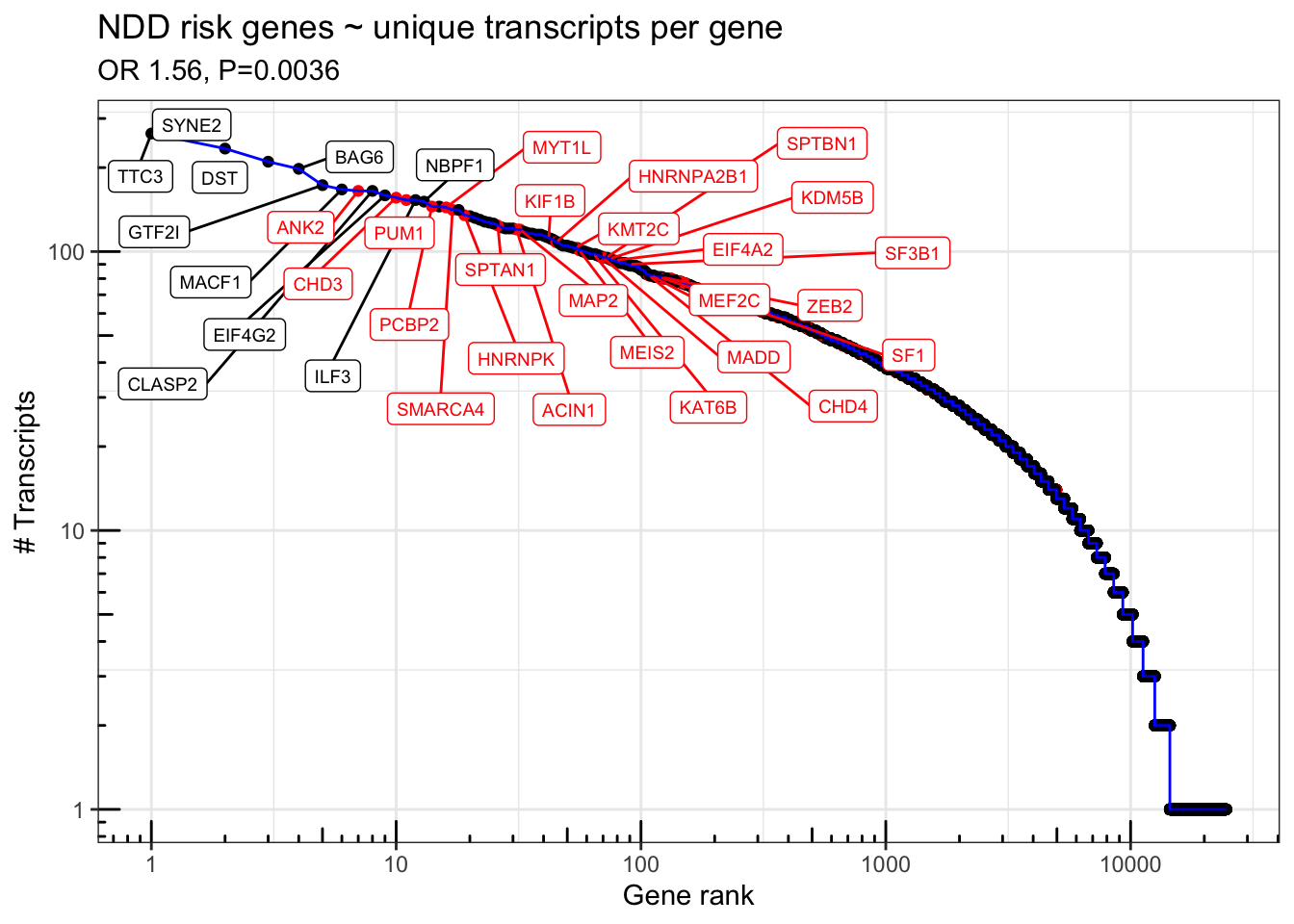
ggsave(file="output/figures/revision1/Fig1K_codingLen_NDD.fuTADA.pdf",Fig1H, width = 8, height=3)FigS3: NDD risk genes ~ unique NOVEL transcipts per gene
df.novel <- talon_gtf %>% as_tibble()  %>% filter(type=="transcript", transcript_id %in% cts$annot_transcript_id[cts$novelty2!="Known"]) %>%
  mutate(gene_id = str_sub(gene_id, 1, 15)) %>%
  group_by(gene_id) %>%
  summarize(n_transcripts = n_distinct(na.omit(transcript_id)), n_exons = n_distinct(na.omit(exon_id))) %>%
  ungroup()

df.novel <- as_tibble(gencode_gtf) %>% dplyr::filter(type=="gene") %>% mutate(gene_id=substr(gene_id,0,15)) %>% right_join(df.novel, by="gene_id")
df.novel <- df.novel %>% left_join(geneCounts)
Joining, by = "gene_id"df.novel <- df.novel %>% left_join(geneLengths)Joining, by = "gene_id"df.novel$gene_rank = rank(-df.novel$n_transcripts, ties.method = 'first')
df.novel$DDD = FALSE
df.novel$DDD[df.novel$gene_name %in% c(asd_genes, ddd_genes)] = TRUE
df.novel = rareVar.binary %>% as_tibble(rownames = "gene_id") %>% right_join(df.novel)Joining, by = "gene_id"s=summary(glm(NDD.fuTADA ~ log10(n_transcripts) + log10(width) + log10(gene_count) + log10(coding_length), data=df.novel %>% filter(gene_type == "protein_coding"), family='binomial'))
print(s)
Call:
glm(formula = NDD.fuTADA ~ log10(n_transcripts) + log10(width) +
    log10(gene_count) + log10(coding_length), family = "binomial",
    data = df.novel %>% filter(gene_type == "protein_coding"))

Deviance Residuals:
    Min       1Q   Median       3Q      Max
-1.1343  -0.4124  -0.3188  -0.2344   3.1335

Coefficients:
                      Estimate Std. Error z value Pr(>|z|)
(Intercept)          -11.16258    0.70920 -15.740  < 2e-16 ***
log10(n_transcripts)   0.37199    0.12866   2.891 0.003837 **
log10(width)           0.53523    0.09565   5.596 2.20e-08 ***
log10(gene_count)      0.34925    0.08999   3.881 0.000104 ***
log10(coding_length)   1.30727    0.22199   5.889 3.89e-09 ***
---
Signif. codes:  0 '***' 0.001 '**' 0.01 '*' 0.05 '.' 0.1 ' ' 1

(Dispersion parameter for binomial family taken to be 1)

    Null deviance: 5174.0  on 10453  degrees of freedom
Residual deviance: 4808.2  on 10449  degrees of freedom
  (751 observations deleted due to missingness)
AIC: 4818.2

Number of Fisher Scoring iterations: 6sort(exp(s$coefficients[,1])) (Intercept) log10(gene_count) log10(n_transcripts)
1.419559e-05 1.418007e+00 1.450619e+00
log10(width) log10(coding_length)
1.707839e+00 3.696057e+00 FigS3 = df.novel %>% mutate(NDD.fuTADA = NDD.fuTADA %>% as.logical() %>% replace_na(F)) %>%
ggplot(aes(x = gene_rank, y = n_transcripts, color=NDD.fuTADA)) +
geom_point() + geom_line(color='blue') +
geom_label_repel(data = . %>% filter(n_transcripts > 150 | (n_transcripts > 75 & NDD.fuTADA==TRUE)),aes(label = gene_name),force = 30, direction='both',nudge_y=-.1,nudge_x = .3, max.iter = 10000,max.overlaps = 50, size=2.5) + scale_color_manual(values=c("TRUE" = "red", "FALSE" = "black")) + scale_y_log10() + scale_x_log10() + theme_bw() + annotation_logticks() + theme(legend.position = 'none') + labs(x="Gene rank", y="# Transcripts") + ggtitle("NDD risk genes ~ unique novel transcripts per gene",subtitle=paste0("OR ",signif(exp(s$coefficients[2,1]),3),", P=", signif(s$coefficients[2,4],2)))
FigS3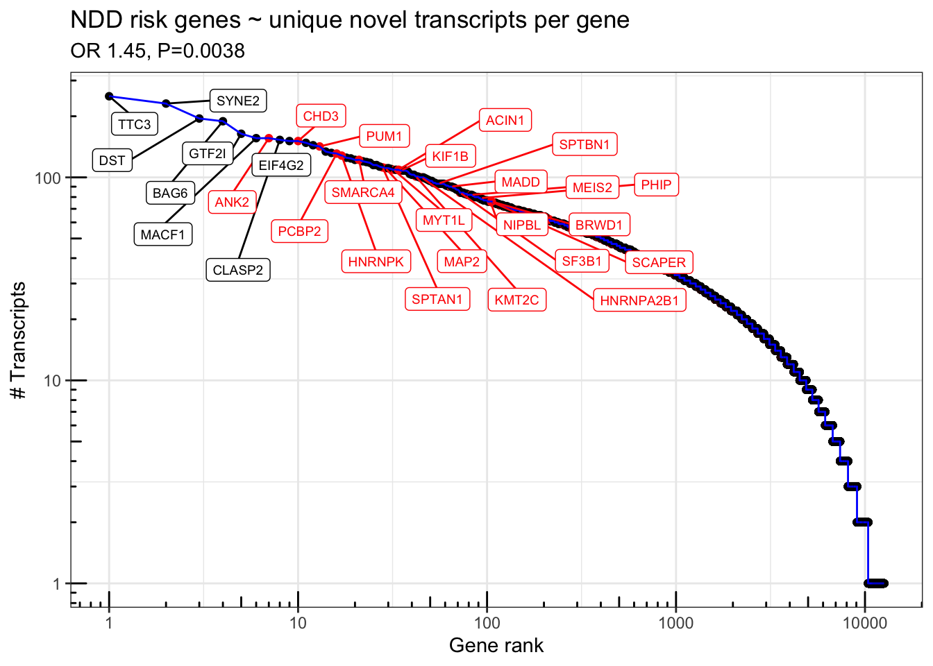
ggsave(file="output/figures/revision1/FigS3G_codingLen_NDD.fuTADA_6in.pdf",FigS3, width = 6, height=3)Pathway Analysis
sumstats <- tx.isoseq %>% group_by(gene_name, gene_type) %>% summarise(total = n_distinct(transcript_id), known = sum(transcript_status=="KNOWN"), ISM.pre = sum(ISM.prefix_transcript=="TRUE", na.rm=T), ISM.suffix = sum(ISM.suffix_transcript=="TRUE", na.rm=T), NIC = sum(NIC_transcript==TRUE, na.rm = T), NNC = sum(NNC_transcript==TRUE, na.rm = T))`summarise()` has grouped output by 'gene_name'. You can override using the
`.groups` argument.write.csv(file="output/isoformNovetyCounts_at_geneLevel.csv",sumstats)
query = sort(unique(tx.isoseq$gene_name[tx.isoseq$transcript_status=="NOVEL" & (tx.isoseq$NNC_transcript==TRUE | tx.isoseq$NIC_transcript == TRUE)]))
bg = sort(unique(tx.isoseq$gene_name[tx.isoseq$transcript_status=="NOVEL" | tx.isoseq$transcript_status=="KNOWN"]))
go = gprofiler2::gost(query = query,custom_bg = bg,sources = c("GO", "KEGG", "REACTOME"),as_short_link = T)Detected custom background input, domain scope is set to 'custom'Gene Body Coverage
files = dir(path = "data/QC/RNA_Metrics/", pattern="RNA_Metrics")
df_coverage_isoseq = data.frame(Position=seq(0,100))

for(i in 1:length(files)) {
  this_file = data.table::fread(paste0("data/QC/RNA_Metrics/", files[i]),skip=10)
  names(this_file)[2] = gsub(".RNA_Metrics", "", files[i])
  df_coverage_isoseq = cbind(df_coverage_isoseq, this_file[,2])
}

files = dir(path = "data/QC/RNA_Metrics_short_read//", pattern="RNA_Metrics")
df_coverage_shortread = data.frame(Position=seq(0,100))

for(i in 1:length(files)) {
  this_file = data.table::fread(paste0("data/QC/RNA_Metrics_short_read/", files[i]),skip=10)
  names(this_file)[2] = gsub(".RNA_Metrics", "", files[i])
  df_coverage_shortread = cbind(df_coverage_shortread, this_file[,2])
}


df_coverage_isoseq <- df_coverage_isoseq %>% pivot_longer(cols = -Position, names_to = "Sample", values_to = "Normalized_coverage")
df_coverage_isoseq$modality = "IsoSeq"

df_coverage_shortread <- df_coverage_shortread %>% pivot_longer(cols = -Position, names_to = "Sample", values_to = "Normalized_coverage")
df_coverage_shortread$modality = "short-read\nRNAseq\n(ribozero)"

ggplot(rbind(df_coverage_isoseq, df_coverage_shortread), aes(x=Position,y=Normalized_coverage,group=Sample, color=modality)) + geom_path() + theme_bw() + labs(x="Gene body position (5' -> 3')", y="Normalized coverage")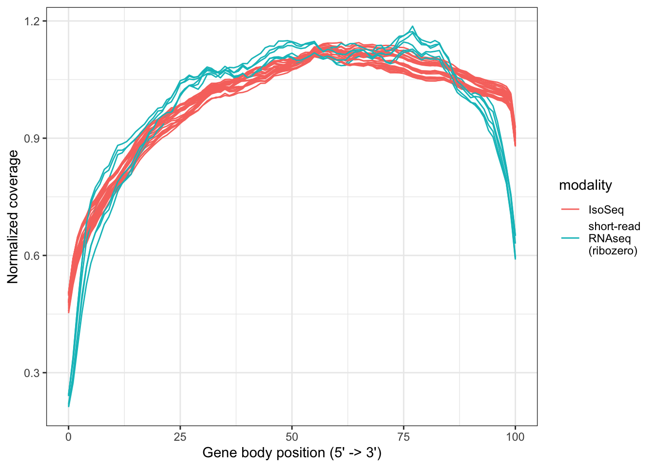
ggsave(file="output/figures/supplement/FigS2A_coverage.pdf",width=5,height=3)