Figure 3 - DTU enrichments

Load Data

suppressPackageStartupMessages({
  library(tidyverse)
  library(rtracklayer)
  library(ggrepel)
  library(biomaRt)
})
knitr::opts_chunk$set(fig.width=12, fig.height=8) 

source("code/fisher_overlap.R")

tableS3.isoform <- read_tsv("output/tables/TableS3_v3.tsv.gz")

Rows: 102319 Columns: 17
── Column specification ────────────────────────────────────────────────────────
Delimiter: "\t"
chr (5): isoform_id, gene_id, gene_name, condition_1, condition_2
dbl (9): DTU_dIF, DTU_pval, DTU_qval, DTE_log2FC, DTE_pval, DTE_qval, DGE_lo...
lgl (3): DTU, DTE, DGE

ℹ Use `spec()` to retrieve the full column specification for this data.
ℹ Specify the column types or set `show_col_types = FALSE` to quiet this message.

tableS3.isoform$ensg = substr(tableS3.isoform$gene_id,1,15)
tableS3.gene <- read_tsv("output/tables/TableS3b_geneLevel.tsv.gz")

Rows: 10809 Columns: 11
── Column specification ────────────────────────────────────────────────────────
Delimiter: "\t"
chr (2): gene_name, gene_id
dbl (6): DTU_qval_min, DTU_pval_min, DTE_qval_min, DTE_pval_min, DGE_pval, D...
lgl (3): DTU, DTE, DGE

ℹ Use `spec()` to retrieve the full column specification for this data.
ℹ Specify the column types or set `show_col_types = FALSE` to quiet this message.

cts = read_table("data/cp_vz_0.75_min_7_recovery_talon_abundance_filtered.tsv.gz")

── Column specification ────────────────────────────────────────────────────────
cols(
  .default = col_double(),
  annot_gene_id = col_character(),
  annot_transcript_id = col_character(),
  annot_gene_name = col_character(),
  annot_transcript_name = col_character(),
  gene_novelty = col_character(),
  transcript_novelty = col_character(),
  ISM_subtype = col_character()
)
ℹ Use `spec()` for the full column specifications.

geneAnno = rtracklayer::import("ref/gencode.v33lift37.annotation.gtf.gz") %>% as_tibble() %>% filter(type=='gene')
geneAnno$ensg = substr(geneAnno$gene_id,1,15)

datAnno = tableS3.isoform %>% mutate(ensg = substr(gene_id,1,15))
datAnno <- datAnno %>% left_join(cts %>% dplyr::select(isoform_id = annot_transcript_id, length))

Joining, by = "isoform_id"

geneSetsForLDSC = data.frame(ensg = unique(datAnno$ensg), set= "background")
geneSetsForLDSC = rbind(geneSetsForLDSC, data.frame(set = "DTU", 
                                   ensg = unique(tableS3.isoform$ensg[tableS3.isoform$DTU ==TRUE])))
geneSetsForLDSC = rbind(geneSetsForLDSC, data.frame(set = "DTU.up", 
                                   ensg = unique(tableS3.isoform$ensg[tableS3.isoform$DTU ==TRUE &
                                                                      tableS3.isoform$DTU_dIF > 0])))
geneSetsForLDSC = rbind(geneSetsForLDSC, data.frame(set = "DTU.down", 
                                   ensg = unique(tableS3.isoform$ensg[tableS3.isoform$DTU ==TRUE &
                                                                      tableS3.isoform$DTU_dIF < 0])))
geneSetsForLDSC = rbind(geneSetsForLDSC, data.frame(set = "DTU.not.DGE", 
                                   ensg = unique(tableS3.isoform$ensg[tableS3.isoform$DTU ==TRUE &
                                                                      tableS3.isoform$DGE == FALSE])))
geneSetsForLDSC = rbind(geneSetsForLDSC, data.frame(set = "DTU.not.DTE", 
                                   ensg = unique(tableS3.isoform$ensg[tableS3.isoform$DTU ==TRUE &
                                                                      tableS3.isoform$DTE == FALSE])))
geneSetsForLDSC = rbind(geneSetsForLDSC, data.frame(set = "DTE", 
                                   ensg = unique(tableS3.isoform$ensg[tableS3.isoform$DTE ==TRUE])))
geneSetsForLDSC = rbind(geneSetsForLDSC, data.frame(set = "DTE.up", 
                                   ensg = unique(tableS3.isoform$ensg[tableS3.isoform$DTE ==TRUE &
                                                                      tableS3.isoform$DTE_log2FC > 0])))
geneSetsForLDSC = rbind(geneSetsForLDSC, data.frame(set = "DTE.down", 
                                   ensg = unique(tableS3.isoform$ensg[tableS3.isoform$DTE ==TRUE &
                                                                      tableS3.isoform$DTE_log2FC < 0])))
geneSetsForLDSC = rbind(geneSetsForLDSC, data.frame(set = "DGE", 
                                   ensg = unique(tableS3.isoform$ensg[tableS3.isoform$DGE ==TRUE])))
geneSetsForLDSC = rbind(geneSetsForLDSC, data.frame(set = "DGE.up", 
                                   ensg = unique(tableS3.isoform$ensg[tableS3.isoform$DGE ==TRUE &
                                                                      tableS3.isoform$DGE_log2FC > 0])))
geneSetsForLDSC = rbind(geneSetsForLDSC, data.frame(set = "DGE.down", 
                                   ensg = unique(tableS3.isoform$ensg[tableS3.isoform$DGE ==TRUE &
                                                                      tableS3.isoform$DGE_log2FC < 0])))

write_tsv(geneSetsForLDSC, file='output/tables/TableS3_DTU_DGE_DTE_forLDSC.tsv')

geneSetsForLDSC$gene = datAnno$gene_name[match(geneSetsForLDSC$ensg, datAnno$ensg)]
write_tsv(geneSetsForLDSC[,c("gene", "set")], file='output/tables/TableS3_DTU_DGE_DTE_forTransite.tsv')

Fig3d: DTU pathway

DTU <- tableS3.gene %>% filter(DTU==T) %>% arrange(DTU_qval_min) %>% dplyr::select(gene_id) %>% pull() %>% substr(0,15)
DTU.bg = tableS3.isoform%>% dplyr::select(gene_id)%>% unique() %>% pull() %>% substr(0,15)

## Pathway analysis with gProfileR
## Note: ordered query here because genes are ranked by DTU significance. Usually this will be F
## Always use the matching background gene set
path = gprofiler2::gost(query=DTU,ordered_query = T,correction_method = 'fdr',
                        custom_bg = DTU.bg, sources = c("GO","KEGG", "REACTOME"))

Detected custom background input, domain scope is set to 'custom'

## Filter results for terms between 5-3000 genes. Also here I remove results where a child GO term is also included, just because there were a lot of results. Can remove this 
df_path = as_tibble(path$result) %>% filter(term_size < 3000, path$result$term_size>5) 
df_path <- df_path %>% filter(!term_id %in% unlist(df_path$parents))

## Plot top 5 results per database
Fig3d <- df_path %>% group_by(source) %>% slice_min(p_value,n=5,with_ties = T) %>% ungroup() %>%
  ggplot(aes(x=reorder(term_name, -p_value), y=-log10(p_value), fill=source)) + geom_bar(stat='identity',position=position_identity()) + coord_flip() + theme_bw() + labs(x="")  + 
  facet_grid(source~., space = 'free', scales='free') + theme(legend.position = 'none')
Fig3d

#ggsave(Fig3d, file="output/figures/Fig3d.pdf",width=4.5,height=3)

DTU.up and DTU.down

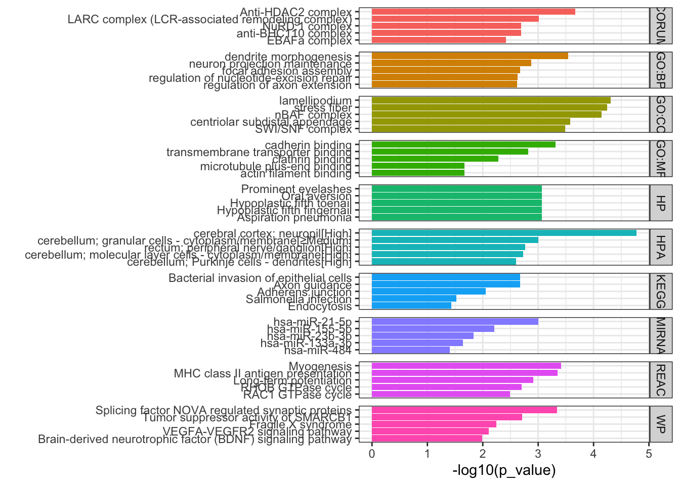
DTU.up <- tableS3.isoform %>%  filter(DTU_dIF > 0, DTU_qval < .05)  %>% arrange(DTU_qval) %>% 
  dplyr::select(gene_id)%>% unique() %>% pull() %>% substr(0,15) 

DTU.down <- tableS3.isoform %>%  filter(DTU_dIF < 0, DTU_qval < .05)  %>% arrange(DTU_qval) %>% 
  dplyr::select(gene_id)%>% unique() %>% pull() %>% substr(0,15)

DTU.bg = tableS3.isoform  %>% arrange(DTU_qval) %>% dplyr::select(gene_id)%>% unique() %>% pull() %>% substr(0,15)

## Pathway analysis with gProfileR
## Note: ordered query here because genes are ranked by DTU significance. Usually this will be F
## Always use the matching background gene set
path.up = gprofiler2::gost(query=DTU.up,ordered_query = T,correction_method = 'fdr',
                        custom_bg = DTU.bg, sources = c("GO","KEGG", "REACTOME", "CORUM", "WP"))

Detected custom background input, domain scope is set to 'custom'

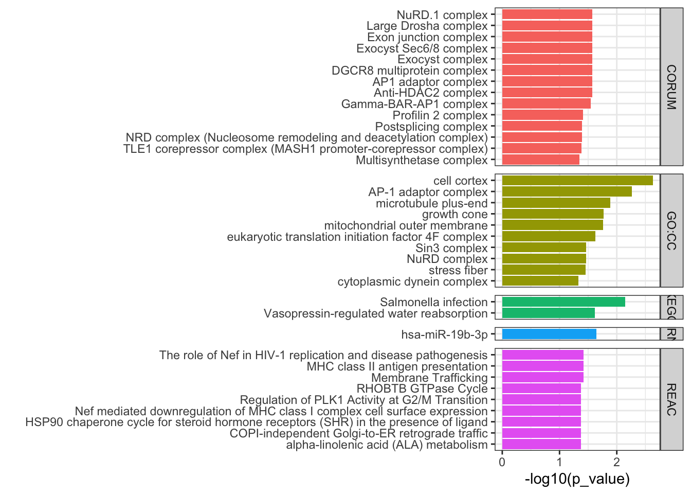
## Filter results for terms between 5-3000 genes. Also here I remove results where a child GO term is also included, just because there were a lot of results. Can remove this 
df_path.up = as_tibble(path.up$result) %>% filter(term_size < 3000, term_size>5) %>% mutate(direction='up')
df_path.up <- df_path.up %>% filter(!term_id %in% unlist(df_path.up$parents))

## Plot top 5 results per database
Fig3d.up <- df_path.up %>% group_by(source) %>% slice_min(p_value,n=8) %>% ungroup() %>%
  ggplot(aes(x=reorder(term_name, -p_value), y=-log10(p_value), fill=source)) + geom_bar(stat='identity', position=position_identity()) + coord_flip() + theme_bw() + labs(x="")  + ggtitle("DTU.up") +
  facet_grid(source~., space = 'free', scales='free') + theme(legend.position = 'none')


path.down = gprofiler2::gost(query=DTU.down,ordered_query = T,correction_method = 'fdr',
                        custom_bg = DTU.bg, sources = c("GO","KEGG", "REACTOME"))

Detected custom background input, domain scope is set to 'custom'

## Filter results for terms between 5-3000 genes. Also here I remove results where a child GO term is also included, just because there were a lot of results. Can remove this 
df_path.down = as_tibble(path.down$result) %>% filter(term_size < 3000, term_size>5)  %>% mutate(direction='down')
df_path.down <- df_path.down %>% filter(!term_id %in% unlist(df_path$parents))

## Plot top 5 results per database
Fig3d.down <- df_path.down %>% group_by(source) %>% slice_min(p_value,n=8) %>% ungroup() %>%
  ggplot(aes(x=reorder(term_name, -p_value), y=-log10(p_value), fill=source)) + geom_bar(stat='identity', position=position_identity()) + coord_flip() + theme_bw() + labs(x="")  + ggtitle("DTU.down") +
  facet_grid(source~., space = 'free', scales='free') + theme(legend.position = 'none')

cowplot::plot_grid(Fig3d.down, Fig3d.up,ncol=2)

DTU all pathways

DTU <- tableS3.gene %>% filter(DTU==T) %>% arrange(DTU_qval_min) %>% dplyr::select(gene_id) %>% pull() %>% substr(0,15)
DTU.bg = tableS3.gene%>% dplyr::select(gene_id)%>% pull() %>% substr(0,15)
path = gprofiler2::gost(query=DTU,ordered_query = T,correction_method = 'fdr',
                        custom_bg = DTU.bg)

Detected custom background input, domain scope is set to 'custom'

df_path = as_tibble(path$result) %>% filter(term_size < 3000, path$result$term_size>5) 
df_path <- df_path %>% filter(!term_id %in% unlist(df_path$parents))

df_path %>% group_by(source) %>% slice_min(p_value,n=5,with_ties = F) %>% ungroup() %>%
  ggplot(aes(x=reorder(term_name, -p_value), y=-log10(p_value), fill=source)) + geom_bar(stat='identity', position=position_identity()) + coord_flip() + theme_bw() + labs(x="")  + 
  facet_grid(source~., space = 'free', scales='free') + theme(legend.position = 'none')

Also: DTU not DGE pathway

DTU <- tableS3.gene %>% filter(DTU==T, DGE_pval>.05) %>% arrange(DTU_qval_min) %>% dplyr::select(gene_id) %>% pull() %>% substr(0,15)
DTU.bg = tableS3.gene%>% dplyr::select(gene_id)%>% pull() %>% substr(0,15)
path = gprofiler2::gost(query=DTU,ordered_query = T,correction_method = 'fdr',
                        custom_bg = DTU.bg)

Detected custom background input, domain scope is set to 'custom'

df_path = as_tibble(path$result) %>% filter(term_size < 3000, path$result$term_size>5) 
df_path <- df_path %>% filter(!term_id %in% unlist(df_path$parents))

df_path %>% group_by(source) %>% slice_min(p_value,n=30) %>% ungroup() %>%
  ggplot(aes(x=reorder(term_name, -p_value), y=-log10(p_value), fill=source)) + geom_bar(stat='identity') + coord_flip() + theme_bw() + labs(x="")  + 
  facet_grid(source~., space = 'free', scales='free') + theme(legend.position = 'none')

EWCE

Using fisher ORA instead

if(FALSE) {
  load("ref/EWCE/CellTypeData_DamonNeuralFetalOnly.rda")
  DTU.up <- tableS3.isoform %>%  filter(DTU_dIF > 0, DTU_qval < .05)  %>% arrange(DTU_qval) %>% 
    dplyr::select(gene_name)%>% unique() %>% pull() %>% substr(0,15) 
  DTU.down <- tableS3.isoform %>%  filter(DTU_dIF < 0, DTU_qval < .05)  %>% arrange(DTU_qval) %>% 
    dplyr::select(gene_name)%>% unique() %>% pull() %>% substr(0,15)
  DTU = unique(c(DTU.up, DTU.down))
  DTU.notDGE <- tableS3.gene %>% filter(DTU==T, DGE_pval>.05) %>% arrange(DTU_qval_min) %>% dplyr::select(gene_name) %>% pull() %>% substr(0,15)
  DTU.bg = tableS3.isoform  %>% arrange(DTU_qval) %>% dplyr::select(gene_name)%>% unique() %>% pull() 
  
  gene_sets = list(DTU,DTU.notDGE)
  names(gene_sets) = c("DTU", "DTU.notDGE")
  df_ewce = data.frame()
  
  for(i in 1:length(gene_sets)) {
    print(i)
    these_genes = gene_sets[[i]]
    
    res=EWCE::bootstrap_enrichment_test(ctd, hits = these_genes, bg=DTU.bg,
                                        genelistSpecies = 'human',sctSpecies = 'human',
                                        annotLevel =2,verbose = F,no_cores = 10)
    df_ewce = rbind(df_ewce,data.frame(list=names(gene_sets)[i], res$results))
  }
  
  
  df_ewce$label = signif(-log10(df_ewce$q+1e-5),2)
  df_ewce$label[df_ewce$q>.05] = ""
  ggplot(df_ewce, aes(x=factor(list),y=CellType, label=label, fill=(sd_from_mean))) + geom_tile() + scale_fill_gradient(low='white', high='red') + geom_text() + theme(axis.text.x = element_text(angle=-45,hjust=0)) + scale_fill_gradient2()

}

Cell-type makers

# Load poliodakis et al markers (Table S4)
# see: https://doi.org/10.1016/j.neuron.2019.06.011
celltypemarkers <- openxlsx::read.xlsx('https://www.cell.com/cms/10.1016/j.neuron.2019.06.011/attachment/508ae008-b926-487a-b871-844a12acc1f8/mmc5', sheet='Cluster enriched genes') %>% as_tibble()
celltypemarkers.tableS5 = openxlsx::read.xlsx('https://www.cell.com/cms/10.1016/j.neuron.2019.06.011/attachment/ec1863fa-0dfc-405c-928c-c5ca96115667/mmc6', sheet='Sub-cluster enriched genes') %>% as_tibble()
celltypemarkers.bg = read.csv("ref/polioudakis_neuron2020/single_cell_background_MJG221228.csv")
celltypemarkers.bg = unique(celltypemarkers.bg$ensembl_gene_id)

DTU <- tableS3.gene %>% filter(DTU==T) %>% arrange(DTU_qval_min) %>% dplyr::select(gene_id) %>% pull() %>% substr(0,15)
DTE <- tableS3.gene %>% filter(DTE==T) %>% arrange(DTU_qval_min) %>% dplyr::select(gene_id) %>% pull() %>% substr(0,15)
DTU_notDGE <- tableS3.gene %>% filter(DTU==T, DGE_pval>.05) %>% arrange(DTU_qval_min) %>% dplyr::select(gene_id) %>% pull() %>% substr(0,15)
DGE <- tableS3.gene %>% filter(DGE==T) %>% arrange(DTU_qval_min) %>% dplyr::select(gene_id) %>% pull() %>% substr(0,15)
DTU_up <- tableS3.isoform %>% filter(DTU==T,DTU_dIF>0) %>% arrange(DTU_qval) %>% dplyr::select(gene_id) %>% unique() %>% pull() %>% substr(0,15)
DTU_down <- tableS3.isoform %>% filter(DTU==T,DTU_dIF<0) %>% arrange(DTU_qval) %>% dplyr::select(gene_id) %>% unique() %>% pull() %>% substr(0,15)

DTU.bg = tableS3.gene%>% dplyr::select(gene_id)%>% pull() %>% substr(0,15)


  df_fisher = data.frame()
  
  for(this_cell in unique(celltypemarkers$Cluster)) {
    marker_genes = celltypemarkers %>% filter(Cluster == this_cell) %>% dplyr::select(Ensembl) %>% pull()
    enrichment = ORA(DTU, marker_genes, DTU.bg, celltypemarkers.bg)
    df_fisher = rbind(df_fisher, data.frame(set="DTU", cell=this_cell, as.data.frame(t(enrichment))))
    
    enrichment2 = ORA(DTU_notDGE, marker_genes, DTU.bg, celltypemarkers.bg)
    df_fisher = rbind(df_fisher, data.frame(set="DTU-not-DGE", cell=this_cell, as.data.frame(t(enrichment2))))
    
     enrichment3 = ORA(DGE, marker_genes, DTU.bg, celltypemarkers.bg)
     df_fisher = rbind(df_fisher, data.frame(set="DGE", cell=this_cell, as.data.frame(t(enrichment3))))

     enrichment4 = ORA(DTE, marker_genes, DTU.bg, celltypemarkers.bg)
     df_fisher = rbind(df_fisher, data.frame(set="DTE", cell=this_cell, as.data.frame(t(enrichment4))))
    # 
    # enrichment5 = ORA(DTU_down, marker_genes, DTU.bg, celltypemarkers.bg)
    # df_fisher = rbind(df_fisher, data.frame(set="DTU_down", cell=this_cell, as.data.frame(t(enrichment5))))
  }
  
  df_fisher$Fisher.p = p.adjust(as.numeric(df_fisher$Fisher.p),'fdr')
  df_fisher$OR = as.numeric(df_fisher$OR)
  
  df_fisher$CellClass = "Other"
  df_fisher$CellClass[grep("Ex",df_fisher$cell)] = "Excitatory Neurons"
  df_fisher$CellClass[grep("In",df_fisher$cell)] = "Interneurons"
  df_fisher$CellClass[df_fisher$cell %in% c("vRG", "oRG", "IP", "PgS", "PgG2M")] = "Progenitors"
  
  Fig3f=ggplot(df_fisher,aes(x=reorder(cell, -Fisher.p), y= -log10(Fisher.p), size=OR, color=-log10(Fisher.p))) +
    geom_point() + coord_flip() + facet_grid(CellClass~set, scales = 'free', space='free_y') + theme_bw() +
    geom_hline(yintercept = 1,lty=2,color='red') + labs(y='Enrichment (-log10 q-value)',x='')
  Fig3f

  ggsave(Fig3f, file="output/figures/Fig3/Fig3f.pdf",width=5,height=4)
  

Fig3f.2 = ggplot(df_fisher,aes(x=reorder(cell, -Fisher.p), y= -log10(Fisher.p), size=OR, color= set)) +
    geom_point() + coord_flip() + facet_grid(CellClass~., scales = 'free', space='free_y') + theme_bw() +
    geom_hline(yintercept = 1,lty=2,color='red') + labs(y='Enrichment (-log10 q-value)',x='')

ggsave(Fig3f.2, file="output/figures/Fig3/Fig3f_2.pdf",width=4,height=6)

Rare variant logit

Isoform-level

using gene level results to be most comparable to DGE

if(FALSE) {

  
  fu=openxlsx::read.xlsx(('https://static-content.springer.com/esm/art%3A10.1038%2Fs41588-022-01104-0/MediaObjects/41588_2022_1104_MOESM3_ESM.xlsx'),'Supplementary Table 11')
  fu$p_TADA_ASD[fu$p_TADA_ASD==0] = min(fu$p_TADA_ASD[fu$p_TADA_ASD >0],na.rm=T)
  fu$p_TADA_NDD[fu$p_TADA_NDD==0] = min(fu$p_TADA_NDD[fu$p_TADA_NDD >0],na.rm=T)
  
  datAnno.logit = data.frame(ASD_fuTADA= -log10(fu$p_TADA_ASD)[match(datAnno$ensg, fu$gene_id)])
  datAnno.logit$NDD_fuTADA = -log10(fu$p_TADA_NDD)[match(datAnno$ensg, fu$gene_id)]
  
  SCZ.schema = read_tsv('ref/risk_genes/SCHEMA_gene_results.tsv')
  datAnno.logit$SCZ_schema = -log10(SCZ.schema$`P meta`[match(datAnno$ensg, SCZ.schema$gene_id)])
  
  BIP.bipex = read_tsv('ref/risk_genes/BipEx_gene_results.tsv') %>% filter(group=="Bipolar Disorder")
  datAnno.logit$BIP.bipex = -log10(BIP.bipex$ptv_fisher_gnom_non_psych_pval[match(datAnno$ensg,BIP.bipex$gene_id)])
  
  EPI.epi25 = read_tsv('ref/risk_genes/Epi25_gene_results.tsv')  %>% group_by(gene_id) %>% summarise(pval = min(pval))
  datAnno.logit$EPI.epi25 = -log10(EPI.epi25$pval[match(datAnno$ensg,EPI.epi25$gene_id)])
  
  
  df_logit= data.frame()
  binaryVec = list("DTU" = as.numeric(datAnno$DTU_qval<.05), "DTE" = as.numeric(datAnno$DTE_qval<.05),
                   "DTU_up" = as.numeric(datAnno$DTU_qval<.05 & datAnno$DTU_dIF>0),
                   "DTU_down" = as.numeric(datAnno$DTU_qval<.05 & datAnno$DTU_dIF<0),
                   "DTE_up" = as.numeric(datAnno$DTE_qval<.05 & datAnno$DTE_log2FC>0),
                   "DTE_down" = as.numeric(datAnno$DTE_qval<.05 & datAnno$DTE_log2FC<0),
                   "DTU_notDGE" = as.numeric(datAnno$DTU_qval<.05 & datAnno$DGE_pval>0.05))
      
  for(i in 1:length(binaryVec)) {
    for(this_rare_var in colnames(datAnno.logit)) {
      this_glm = summary(glm(binaryVec[[i]] ~ datAnno.logit[,this_rare_var] + length + log10(length), data=datAnno, family='binomial'))
      df_logit = rbind(df_logit, data.frame(feature = names(binaryVec)[[i]], set = this_rare_var, t(this_glm$coefficients[2,])))
  }}
      
  df_logit$OR = exp(df_logit$Estimate)
  df_logit$P = df_logit$Pr...z..
  df_logit$P[df_logit$OR < 1] = 1
  df_logit$Q = p.adjust(df_logit$P,'fdr')
  df_logit$class = "DGE"
  df_logit$class[grepl("DTE", df_logit$feature)] = "DTE"
  df_logit$class[grepl("DTU", df_logit$feature)] = "DTU"
  
  
  ggplot(df_logit, aes(x=reorder(set,-Q), y=-log10(Q), fill=OR)) + geom_bar(stat='identity') + 
    coord_flip() + geom_hline(yintercept = 1, lty=2,col='red') + labs(y="-log10(qvalue)",x="") + theme_bw() + facet_wrap(feature~.,ncol = 3)
  
  
  g1 = ggplot(df_logit %>% filter(feature %in% c("DTU", "DTE", "DTU_notDGE")), aes(x=reorder(set,-Q), y=-log10(Q), fill=OR)) + geom_bar(stat='identity') + 
    coord_flip() + geom_hline(yintercept = 1, lty=2,col='red') + labs(y="-log10(qvalue)",x="") + theme_bw() + facet_grid(feature~.)
}

Gene-level

tableS3.isoform$ensg = substr(tableS3.isoform$gene_id,1,15)

datAnno = tableS3.gene %>% mutate(ensg = substr(gene_id,1,15))
datAnno <- datAnno %>% left_join(geneAnno %>% dplyr::select(ensg, length=width))

Joining, by = "ensg"

fu=openxlsx::read.xlsx(('https://static-content.springer.com/esm/art%3A10.1038%2Fs41588-022-01104-0/MediaObjects/41588_2022_1104_MOESM3_ESM.xlsx'),'Supplementary Table 11')
fu$p_TADA_ASD[fu$p_TADA_ASD==0] = min(fu$p_TADA_ASD[fu$p_TADA_ASD >0],na.rm=T)
fu$p_TADA_NDD[fu$p_TADA_NDD==0] = min(fu$p_TADA_NDD[fu$p_TADA_NDD >0],na.rm=T)

datAnno.logit = data.frame(ASD_fuTADA= -log10(fu$p_TADA_ASD)[match(datAnno$ensg, fu$gene_id)])
datAnno.logit$NDD_fuTADA = -log10(fu$p_TADA_NDD)[match(datAnno$ensg, fu$gene_id)]

SCZ.schema = read_tsv('ref/risk_genes/SCHEMA_gene_results.tsv')

Warning: One or more parsing issues, see `problems()` for details

Rows: 18321 Columns: 26
── Column specification ────────────────────────────────────────────────────────
Delimiter: "\t"
chr  (8): gene_id, group, OR (PTV), OR (Class I), OR (Class II), OR (PTV) up...
dbl (16): Case PTV, Ctrl PTV, Case mis3, Ctrl mis3, Case mis2, Ctrl mis2, P ...
lgl  (2): De novo mis3, De novo mis2

ℹ Use `spec()` to retrieve the full column specification for this data.
ℹ Specify the column types or set `show_col_types = FALSE` to quiet this message.

datAnno.logit$SCZ_schema = -log10(SCZ.schema$`P meta`[match(datAnno$ensg, SCZ.schema$gene_id)])

BIP.bipex = read_tsv('ref/risk_genes/BipEx_gene_results.tsv') %>% filter(group=="Bipolar Disorder")

Rows: 119958 Columns: 20
── Column specification ────────────────────────────────────────────────────────
Delimiter: "\t"
chr  (4): gene_id, group, damaging_missense_fisher_gnom_non_psych_OR, ptv_fi...
dbl (16): n_cases, n_controls, damaging_missense_case_count, damaging_missen...

ℹ Use `spec()` to retrieve the full column specification for this data.
ℹ Specify the column types or set `show_col_types = FALSE` to quiet this message.

datAnno.logit$BIP.bipex = -log10(BIP.bipex$ptv_fisher_gnom_non_psych_pval[match(datAnno$ensg,BIP.bipex$gene_id)])

EPI.epi25 = read_tsv('ref/risk_genes/Epi25_gene_results.tsv')  %>% group_by(gene_id) %>% summarise(pval = min(pval))

Rows: 71456 Columns: 12
── Column specification ────────────────────────────────────────────────────────
Delimiter: "\t"
chr (2): gene_id, group
dbl (9): xcase_lof, xctrl_lof, pval_lof, xcase_mpc, xctrl_mpc, pval_mpc, xca...
lgl (1): pval_infrIndel

ℹ Use `spec()` to retrieve the full column specification for this data.
ℹ Specify the column types or set `show_col_types = FALSE` to quiet this message.

datAnno.logit$EPI.epi25 = -log10(EPI.epi25$pval[match(datAnno$ensg,EPI.epi25$gene_id)])


df_logit= data.frame()
binaryVec = list("DTU" = as.numeric(datAnno$DTU), "DTE" = as.numeric(datAnno$DTE), "DGE"=as.numeric(datAnno$DGE),
                 "DTU-not-DGE" = as.numeric(datAnno$DTU & !datAnno$DGE), 
                 "DTU-not-DTE" = as.numeric(datAnno$DTU & !datAnno$DTE),
                 "DTU.up" = as.numeric(datAnno$ensg %in% (tableS3.isoform %>% filter(DTU, DTU_dIF>0) %>% dplyr::select(ensg) %>% pull())),
                 "DTU.down" = as.numeric(datAnno$ensg %in% (tableS3.isoform %>% filter(DTU, DTU_dIF<0) %>% dplyr::select(ensg) %>% pull())),
                 "DTE.up" = as.numeric(datAnno$ensg %in% (tableS3.isoform %>% filter(DTE, DTE_log2FC>0) %>% dplyr::select(ensg) %>% pull())),
                 "DTE.down" = as.numeric(datAnno$ensg %in% (tableS3.isoform %>% filter(DTE, DTE_log2FC<0) %>% dplyr::select(ensg) %>% pull())),
                 "DGE.up" = as.numeric(datAnno$ensg %in% (tableS3.isoform %>% filter(DGE, DGE_log2FC>0) %>% dplyr::select(ensg) %>% pull())),
                 "DGE.down" = as.numeric(datAnno$ensg %in% (tableS3.isoform %>% filter(DGE, DGE_log2FC<0) %>% dplyr::select(ensg) %>% pull())))
    
for(i in 1:length(binaryVec)) {
  for(this_rare_var in colnames(datAnno.logit)) {
    this_glm = summary(glm(datAnno.logit[,this_rare_var] ~ binaryVec[[i]] + length + log10(length), data=datAnno))
    df_logit = rbind(df_logit, data.frame(feature = names(binaryVec)[[i]], set = this_rare_var, t(this_glm$coefficients[2,])))
}}
    
df_logit$OR = exp(df_logit$Estimate)
df_logit$P = df_logit$Pr...z..
df_logit$Q = p.adjust(df_logit$P,'fdr')
df_logit$class = "DGE"
df_logit$class[grepl("DTE", df_logit$feature)] = "DTE"
df_logit$class[grepl("DTU", df_logit$feature)] = "DTU"

Fig3H=ggplot(df_logit %>% filter(feature %in% c("DTE", "DGE", "DTU", "DTU-not-DGE")), aes(x=reorder(set,-Q), y=-log10(Q), color=feature, alpha = OR > 1,size=OR)) +
    geom_point() + coord_flip() + geom_hline(yintercept = -log10(.05), lty=2,col='red') +  
  scale_alpha_manual(values = c(.5, 1))+
    labs(y="-log10(qvalue)",x="") + theme_bw() + ggtitle('Gene level rare variant enrichment')

Fig3H

ggsave(Fig3H,file='output/figures/Fig3/Fig3H.pdf',width=5,height=2.5)


df_logit$class[grepl("-not-", df_logit$feature)] = "DTU-not-DGE/DTE"
df_logit$feature = factor(df_logit$feature, levels=c("DGE", "DGE.down", "DGE.up","DTE", "DTE.down", "DTE.up","DTU", "DTU.down", "DTU.up","DTU-not-DGE", "DTU-not-DTE"))

FigS4B=ggplot(df_logit, aes(x=reorder(set,-Q), y=-log10(Q), color=class, size=OR, alpha=OR>1)) + geom_point() + 
  coord_flip() + geom_hline(yintercept = -log10(.05), lty=2,col='red') + labs(y="-log10(qvalue)",x="") + theme_bw() + facet_wrap(feature~.,ncol = 3) + scale_alpha_manual(values = c(.5, 1))
ggsave(FigS4B,file='output/figures/supplement/FigS4B.pdf',width=7,height=5)
FigS4B

# ggplot(df_logit, aes(x=reorder(feature,-Q), y=-log10(Q), fill=OR)) + geom_bar(stat='identity') + 
#   coord_flip() + geom_hline(yintercept = -log10(.05), lty=2,col='red') + labs(y="-log10(qvalue)",x="") + theme_bw() +   facet_grid(set~.,scales = 'free')

RBP Enrichments

Celine’s RBP Targets

rbp_targets = read.csv("ref/RBPs/RBP_targets_v2.csv")
rbp_targets$regulation[is.na(rbp_targets$regulation)]=""


mart = useMart("ENSEMBL_MART_ENSEMBL","mmusculus_gene_ensembl")
f = listFilters(mart); a = listAttributes(mart)
featuresToGet = c("ensembl_gene_id", "external_gene_name", "hsapiens_homolog_ensembl_gene", "hsapiens_homolog_associated_gene_name","hsapiens_homolog_orthology_type")
mouseHumanHomologs = getBM(attributes = featuresToGet,mart = mart)

human_mouse_bg = mouseHumanHomologs %>% as_tibble() %>% filter(hsapiens_homolog_orthology_type == "ortholog_one2one") %>% dplyr::select("hsapiens_homolog_ensembl_gene") %>% pull()



genesets = list("DTU"= tableS3.gene %>% filter(DTU) %>% mutate(gene_id = substr(gene_id,1,15)) %>% dplyr::select(gene_id) %>% pull(),
                  "DTE" = tableS3.gene %>% filter(DTE) %>% mutate(gene_id = substr(gene_id,1,15)) %>% dplyr::select(gene_id) %>% pull(),
                  "DGE" = tableS3.gene %>% filter(DTE) %>% mutate(gene_id = substr(gene_id,1,15)) %>% dplyr::select(gene_id) %>% pull(),
                  "DTUnotDGE" = tableS3.gene %>% filter(DTU,DGE_pval>.05) %>% mutate(gene_id = substr(gene_id,1,15)) %>% 
                    dplyr::select(gene_id) %>% pull())
DTU.bg = tableS3.gene %>% mutate(gene_id = substr(gene_id,1,15)) %>% dplyr::select(gene_id) %>% pull() %>% unique()

df_fisher = data.frame()
for(i in 1:length(genesets)) {
  for(this_dataset in unique(na.omit(rbp_targets$dataset))) {
    this_rbp = rbp_targets %>% filter(dataset == this_dataset) %>% mutate(target = paste0(RBP, "_", data.type, "_", msORhs)) %>% dplyr::select(target) %>% unique()  %>% pull()
    target_genes = rbp_targets %>% filter(dataset == this_dataset) %>% dplyr::select(ENSG) %>% pull()
 
 if(grepl("Human",this_rbp)) {
   this_or = ORA(genesets[[i]], target_genes, DTU.bg, DTU.bg)
 } else {
  this_or = ORA(genesets[[i]], target_genes, DTU.bg, human_mouse_bg)
 }
 df_fisher = rbind(df_fisher, data.frame(set = names(genesets)[[i]], dataset = this_dataset, target = this_rbp, t(this_or)))
  }
}
  df_fisher$OR = as.numeric(df_fisher$OR)
  df_fisher$Fisher.p[df_fisher$OR<1] = 1
  df_fisher$Fisher.p = p.adjust(as.numeric(df_fisher$Fisher.p),'fdr')
  
  df_fisher$target = factor(df_fisher$target, levels= df_fisher %>% filter(set=="DTU") %>%  group_by(target) %>% summarise(pmin = min(Fisher.p)) %>% arrange(pmin) %>% dplyr::select(target) %>% pull())
  df_fisher$org = "Mouse"; df_fisher$org[grep("Human",df_fisher$target)] = "Human"
  df_fisher$data.type = rbp_targets$data.type[match(df_fisher$dataset, rbp_targets$dataset)]
  df_fisher$cell.type = rbp_targets$cell.type[match(df_fisher$dataset, rbp_targets$dataset)]
  df_fisher$label = signif(df_fisher$OR,1)
  df_fisher$label[df_fisher$Fisher.p>.05] = ''
  Fig3H.1=ggplot(df_fisher %>% filter(set=="DTU"),aes(x=target, y= -log10(Fisher.p), fill=OR)) +
    geom_bar(stat='identity',position = position_dodge2()) + theme_bw() +
    geom_hline(yintercept = 1,lty=2,color='red') + labs(y='Enrichment\n(-log10 q-value)',x='') + theme(axis.text.x = element_text(angle=90,vjust = .5, hjust=1))
  
  ggplot(df_fisher,aes(x=target, y= set, fill=-log10(Fisher.p),label=label)) + geom_tile(color='grey60') + geom_text(size=2) + theme_bw() +
     labs(y='',x='') + theme(axis.text.x = element_text(angle=90,vjust = .5, hjust=1)) + 
    scale_fill_gradient(low='white', high='red')

    Fig3H.2=ggplot(df_fisher %>% filter(set=="DTU"),aes(x=target, label=cell.type)) + geom_tile(aes(y=factor(1),fill=data.type)) + geom_point(aes(y=factor(1), shape=cell.type),position=position_dodge2()) + scale_shape_manual(values = c(1:9)) + theme_bw() + theme(axis.text.x = element_blank()) + labs(x="", y="")
  
    pdf(file="output/figures/Fig3/Fig3H.pdf",width = 8,height=5)
    gridExtra::grid.arrange(grobs=list(Fig3H.1,Fig3H.2),layout_matrix=cbind(c(1,1,1,1,1,1,1,2)))

Warning: Width not defined. Set with `position_dodge2(width = ?)`

  dev.off()

quartz_off_screen 
                2 

  Fig3H_supplement=ggplot(df_fisher,aes(x=reorder(target, -Fisher.p), y= -log10(Fisher.p), fill=OR)) +
    geom_bar(stat='identity',position = position_dodge2()) + coord_flip() + theme_bw() + facet_grid(~set) +
    geom_hline(yintercept = 1,lty=2,color='red') + labs(y='Enrichment (-log10 q-value)',x='')
Fig3H_supplement

ggsave(Fig3H_supplement, file="output/figures/supplement/Fig3H_supp.pdf",width = 8,height=5)

RBP motif:

# library(transite)
# 
# library(biomaRt)
# mart = useMart('ENSEMBL_MART_ENSEMBL', 'hsapiens_gene_ensembl',host = 'https://grch37.ensembl.org')
# a=listAttributes(mart)
# ensembl = getBM(attributes=c("ensembl_gene_id", "hgnc_symbol",'refseq_mrna'),mart=mart)
# 
# 
# out = run_kmer_tsma(foreground_sets = tableS3.gene$gene_name[tableS3.gene$DTU], background_set = tableS3.gene$gene_name)