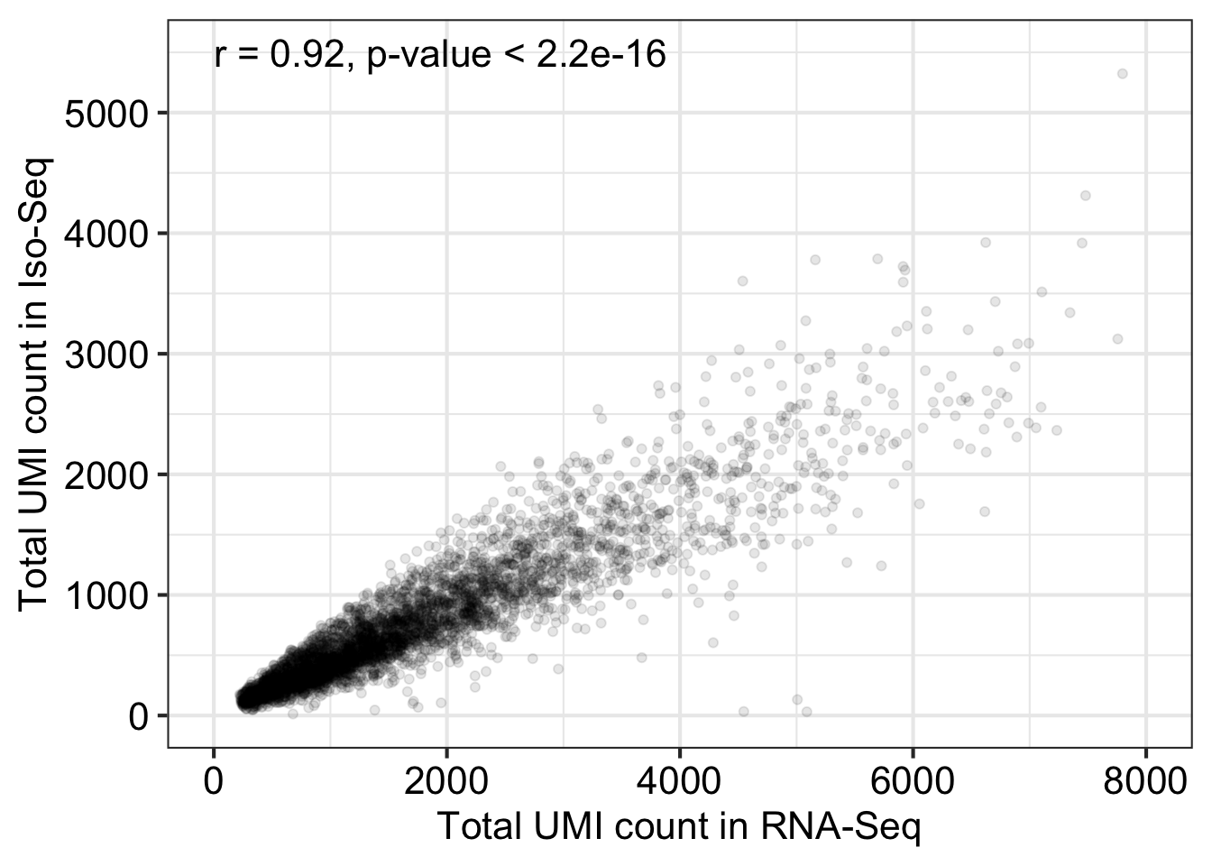
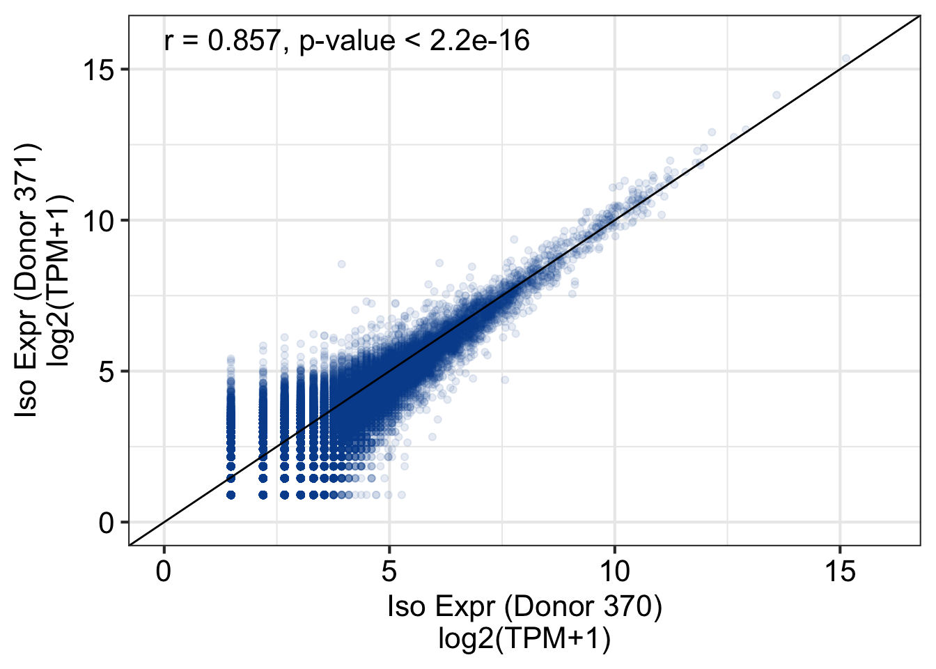
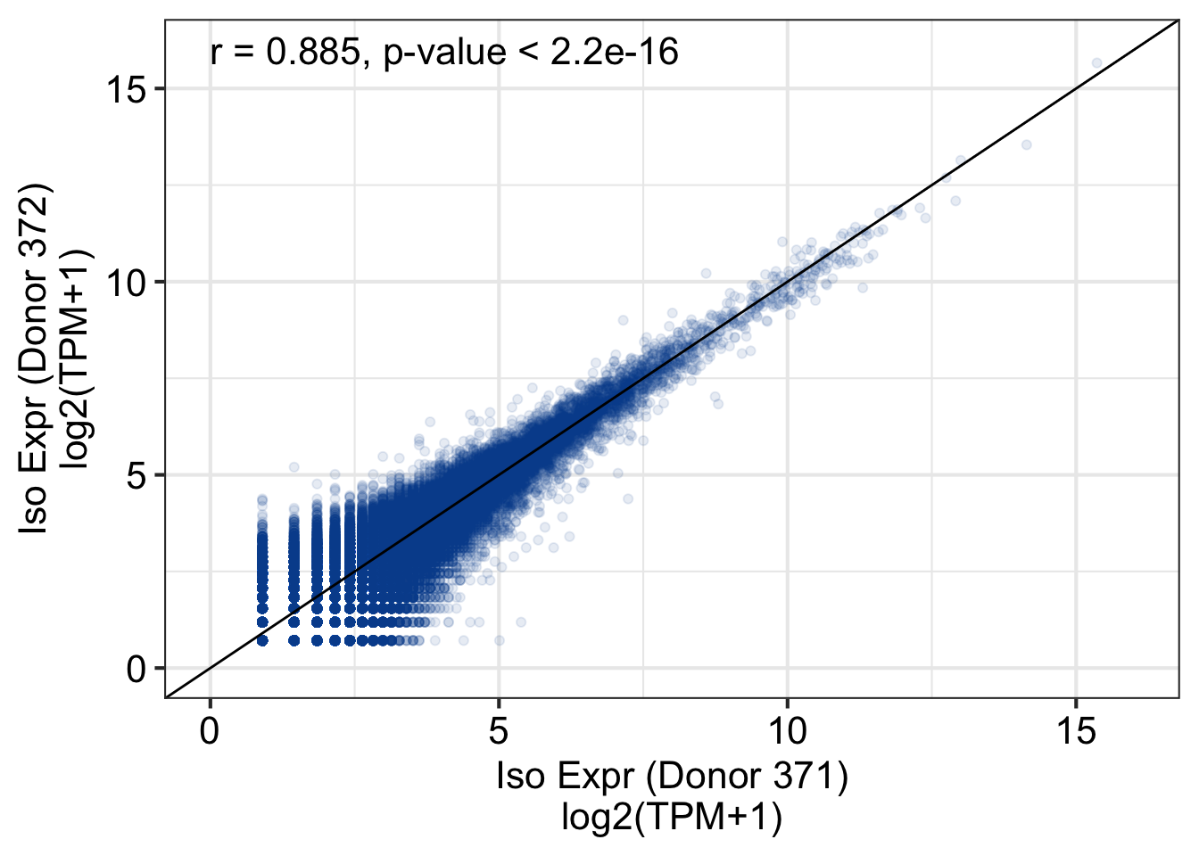
Figure S9 - Correlation plots

library(tidyverse)

── Attaching packages ─────────────────────────────────────── tidyverse 1.3.2 ──
✔ ggplot2 3.3.6      ✔ purrr   0.3.4 
✔ tibble  3.1.8      ✔ dplyr   1.0.10
✔ tidyr   1.2.0      ✔ stringr 1.5.0 
✔ readr   2.1.2      ✔ forcats 0.5.2 
── Conflicts ────────────────────────────────────────── tidyverse_conflicts() ──
✖ dplyr::filter() masks stats::filter()
✖ dplyr::lag()    masks stats::lag()

library(rtracklayer)

Loading required package: GenomicRanges
Loading required package: stats4
Loading required package: BiocGenerics

Attaching package: 'BiocGenerics'

The following objects are masked from 'package:dplyr':

    combine, intersect, setdiff, union

The following objects are masked from 'package:stats':

    IQR, mad, sd, var, xtabs

The following objects are masked from 'package:base':

    anyDuplicated, append, as.data.frame, basename, cbind, colnames,
    dirname, do.call, duplicated, eval, evalq, Filter, Find, get, grep,
    grepl, intersect, is.unsorted, lapply, Map, mapply, match, mget,
    order, paste, pmax, pmax.int, pmin, pmin.int, Position, rank,
    rbind, Reduce, rownames, sapply, setdiff, sort, table, tapply,
    union, unique, unsplit, which.max, which.min

Loading required package: S4Vectors

Attaching package: 'S4Vectors'

The following objects are masked from 'package:dplyr':

    first, rename

The following object is masked from 'package:tidyr':

    expand

The following objects are masked from 'package:base':

    expand.grid, I, unname

Loading required package: IRanges

Attaching package: 'IRanges'

The following objects are masked from 'package:dplyr':

    collapse, desc, slice

The following object is masked from 'package:purrr':

    reduce

Loading required package: GenomeInfoDb

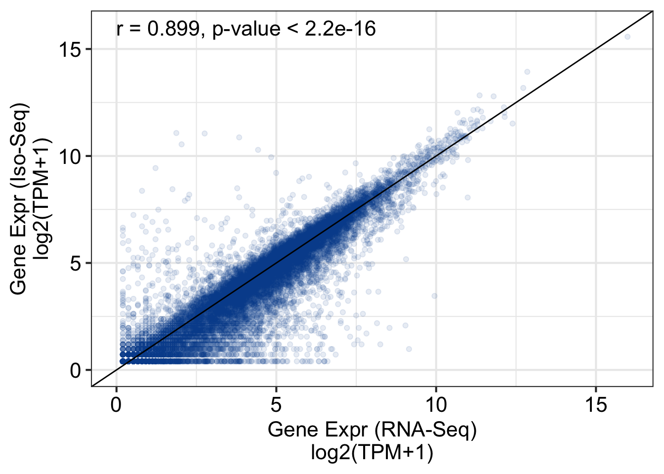
Sys.setenv("VROOM_CONNECTION_SIZE" = 524288) # 512kb - default is 128kb. entire line must fit inside this buffer and we have very long lines

base_size_pt = 16
theme_set(theme_bw(base_size = base_size_pt))
theme_update(
  plot.title = element_text(size = rel(1.2), hjust = 0.5),
  axis.title = element_text(size = rel(1)),
  axis.text = element_text(color="black", size = rel(1)),
  legend.title = element_text(size = rel(1)),
  legend.text = element_text(color="black", size = rel(1)),
  strip.text = element_text(color="black", size = rel(1))
)
base_size_mm = base_size_pt * 25.4 / 72.27

isoseq = read_tsv("data/AllBarcode_newID_geneLevel.txt.gz")

Rows: 19158 Columns: 4282
── Column specification ────────────────────────────────────────────────────────
Delimiter: "\t"
chr    (1): gene_name
dbl (4281): ACGGCATAGTAC, ACTGACTGATCC, ACTGGCACCGAG, AGCTAGCCCATG, AGTTTAGC...

ℹ Use `spec()` to retrieve the full column specification for this data.
ℹ Specify the column types or set `show_col_types = FALSE` to quiet this message.

isoseq

# A tibble: 19,158 × 4,282
   gene_name ACGGCATAG…¹ ACTGA…² ACTGG…³ AGCTA…⁴ AGTTT…⁵ ATCCG…⁶ CAGAC…⁷ CCCCC…⁸
   <chr>           <dbl>   <dbl>   <dbl>   <dbl>   <dbl>   <dbl>   <dbl>   <dbl>
 1 A1BG                0       0       0       0       0       0       0       0
 2 A1BG-AS1            0       0       0       0       0       0       0       0
 3 A2M                 0       0       0       1       0       0       0       0
 4 AAAS                0       0       0       0       0       0       0       0
 5 AACS                1       0       0       0       0       0       0       0
 6 AADAT               0       0       0       0       0       0       0       0
 7 AAGAB               0       0       0       0       0       0       0       0
 8 AAK1                0       0       0       0       0       0       0       0
 9 AAMDC               0       0       0       0       0       0       0       0
10 AAMP                0       0       0       0       0       0       0       0
# … with 19,148 more rows, 4,273 more variables: GCCGTAAAACTC <dbl>,
#   GGGCTGCTTATA <dbl>, GGTTGCTGTACG <dbl>, GTAGCGAGATGC <dbl>,
#   TCAGCTCACCCT <dbl>, TGACATTCTATT <dbl>, TGGTGAACCAGA <dbl>,
#   TTCTATGCCCGC <dbl>, AAAAATAAATTG <dbl>, AAAACCGCGCAG <dbl>,
#   AAAAGCAACGTG <dbl>, AAAGGCGCGCGG <dbl>, AAATCAACTGTA <dbl>,
#   AACCACGTTTAA <dbl>, AACGTACTATCG <dbl>, AACTGCCTTGTA <dbl>,
#   AAGATCCAAGGC <dbl>, AAGGCAGAATCT <dbl>, AAGGCTGACCGA <dbl>, …

short_read = read_tsv("data/single_cell/Raw_Single_Cell_4281.tsv.gz")

Rows: 30119 Columns: 4282
── Column specification ────────────────────────────────────────────────────────
Delimiter: "\t"
chr    (1): gene_name
dbl (4281): GTATAACATGAA, CGAATATTCTGT, TGGAACAGCAAT, TACCCTGTAAGA, CTCACTGA...

ℹ Use `spec()` to retrieve the full column specification for this data.
ℹ Specify the column types or set `show_col_types = FALSE` to quiet this message.

short_read

# A tibble: 30,119 × 4,282
   gene_name GTATAACAT…¹ CGAAT…² TGGAA…³ TACCC…⁴ CTCAC…⁵ ACAGC…⁶ AGTCC…⁷ AGGCT…⁸
   <chr>           <dbl>   <dbl>   <dbl>   <dbl>   <dbl>   <dbl>   <dbl>   <dbl>
 1 TSPAN6              0       1       0       1       0       1       1       0
 2 DPM1                1       0       0       0       0       1       3       2
 3 SCYL3               0       0       0       0       0       0       0       0
 4 C1orf112            0       0       0       0       1       0       1       0
 5 CFH                 0       0       0       0       0       0       0       0
 6 FUCA2               0       0       0       0       0       0       0       0
 7 GCLC                0       0       0       0       0       0       0       0
 8 NFYA                1       0       0       0       0       0       0       0
 9 STPG1               0       0       0       0       0       0       0       0
10 NIPAL3              0       0       0       0       0       0       0       0
# … with 30,109 more rows, 4,273 more variables: CCATCTATCAGG <dbl>,
#   AAGAAGTCCATT <dbl>, GCCGCAGAGTCA <dbl>, AACCTTCGCAAC <dbl>,
#   CTCTCCCCAATC <dbl>, TTTTATTTATAA <dbl>, CGTATCAGTATT <dbl>,
#   GTACTCTACAGA <dbl>, CAGTTTAGGAAA <dbl>, GTACCACCCTTC <dbl>,
#   ATGTGCACAGCA <dbl>, GTAGGTTAACTA <dbl>, CAGGGCCAGGCA <dbl>,
#   CGGGAACCCAAA <dbl>, GTGATTAGCCCA <dbl>, ATCTCCTTGTTA <dbl>,
#   CGGCTTATCGTA <dbl>, ACCCATCAAAGG <dbl>, GGCTGAGAGTCA <dbl>, …

cell_metadata = read_tsv("ref/polioudakis_neuron2020/TableS3_Cell_metadata.csv")

Rows: 33976 Columns: 14
── Column specification ────────────────────────────────────────────────────────
Delimiter: "\t"
chr (7): Cell, Cluster, Subcluster, Layer, Index, Library, Phase
dbl (7): Donor, Gestation_week, Number_genes_detected, Number_UMI, Percentag...

ℹ Use `spec()` to retrieve the full column specification for this data.
ℹ Specify the column types or set `show_col_types = FALSE` to quiet this message.

cell_metadata

# A tibble: 33,976 × 14
   Cell        Cluster Subcl…¹ Donor Layer Gesta…² Index Library Numbe…³ Numbe…⁴
   <chr>       <chr>   <chr>   <dbl> <chr>   <dbl> <chr> <chr>     <dbl>   <dbl>
 1 TGCTAATACT… vRG     vRG_0     368 CP         17 N701  Plath      1366    2736
 2 TTCACGATTT… vRG     vRG_2     368 GZ         17 N702  Plath      3012    7318
 3 CTGTCAGAAT… vRG     vRG_2     368 GZ         17 N702  Plath      1597    3451
 4 CATAATATGT… vRG     vRG_0     368 GZ         17 N702  Plath      1551    2941
 5 TGCCAATCCG… vRG     vRG_0     368 GZ         17 N702  Plath      1569    2769
 6 TCGACTATTT… vRG     vRG_2     368 GZ         17 N702  Plath      1610    2994
 7 GTTACCCGGC… vRG     vRG_1     368 GZ         17 N702  Plath      1227    2092
 8 GCCACCGATA… vRG     vRG_1     368 GZ         17 N702  Plath      1197    2057
 9 GGGCAGATGT… vRG     vRG_1     368 GZ         17 N702  Plath      1237    2221
10 TTGAGCGGTA… vRG     vRG_0     368 GZ         17 N702  Plath      1344    2393
# … with 33,966 more rows, 4 more variables: Percentage_mitochondrial <dbl>,
#   S_phase_score <dbl>, G2M_phase_score <dbl>, Phase <chr>, and abbreviated
#   variable names ¹​Subcluster, ²​Gestation_week, ³​Number_genes_detected,
#   ⁴​Number_UMI

Gene expr

gene_counts = inner_join(
  isoseq %>% mutate(
    cts_isoseq = rowSums(across(where(is.numeric))),
    .keep = "unused"
  ),
  short_read %>% mutate(
    cts_short_read = rowSums(across(where(is.numeric))),
    .keep = "unused"
  ),
  by = "gene_name"
) %>%
  filter(!if_any(starts_with("cts_"), ~.x == 0))
gene_counts

# A tibble: 13,946 × 3
   gene_name cts_isoseq cts_short_read
   <chr>          <dbl>          <dbl>
 1 A1BG              18              6
 2 A1BG-AS1           3              6
 3 A2M               22             57
 4 AAAS             169            288
 5 AACS              69            198
 6 AADAT             79            174
 7 AAGAB             62             82
 8 AAK1              64            479
 9 AAMDC             95            189
10 AAMP             298            401
# … with 13,936 more rows

gene_counts_logRPM = gene_counts %>%
  mutate(across(
    starts_with("cts_"),
    ~log2(1 + (.x / (sum(.x) / 1000000)))
  ))
gene_counts_logRPM

# A tibble: 13,946 × 3
   gene_name cts_isoseq cts_short_read
   <chr>          <dbl>          <dbl>
 1 A1BG           2.77           0.916
 2 A1BG-AS1       0.976          0.916
 3 A2M            3.02           3.24 
 4 AAAS           5.79           5.44 
 5 AACS           4.54           4.92 
 6 AADAT          4.73           4.74 
 7 AAGAB          4.39           3.71 
 8 AAK1           4.43           6.17 
 9 AAMDC          4.98           4.85 
10 AAMP           6.60           5.91 
# … with 13,936 more rows

cor = cor.test(gene_counts_logRPM$cts_isoseq, gene_counts_logRPM$cts_short_read, method = "pearson")
cor

    Pearson's product-moment correlation

data:  gene_counts_logRPM$cts_isoseq and gene_counts_logRPM$cts_short_read
t = 242.12, df = 13944, p-value < 2.2e-16
alternative hypothesis: true correlation is not equal to 0
95 percent confidence interval:
 0.8955646 0.9019444
sample estimates:
      cor 
0.8988021 

ggplot(
  gene_counts_logRPM,
  aes(x = cts_short_read, y = cts_isoseq)
) +
  geom_point(alpha = 0.1, color = "#08519c") +
  geom_abline() +
  annotate(
    geom = "text",
    label = str_c("r = ", round(cor$estimate[[1]], digits = 3), ", p\uadvalue < 2.2e-16"),
    size = base_size_mm,
    x = 0, y = 16,
    vjust = "middle", hjust = "left",
    parse = F
  ) +
  xlim(0, 16) +
  ylim(0, 16) +
  labs(
    x = "Gene Expr (RNA\uadSeq)\nlog2(TPM+1)",
    y = "Gene Expr (Iso\uadSeq)\nlog2(TPM+1)"
  )

ggsave("output/figures/supplement/FigS9_GeneExprCor.pdf", width = 5, height = 5)

UMI

UMI_counts = inner_join(
  short_read %>%
    select(-gene_name) %>%
    summarize(across(everything(), sum)) %>%
    pivot_longer(everything(), names_to = "UMI", values_to = "cts_short_read"),
  isoseq %>%
    select(-gene_name) %>%
    summarize(across(everything(), sum)) %>%
    pivot_longer(everything(), names_to = "UMI", values_to = "cts_isoseq"),
  by = "UMI"
)
UMI_counts

# A tibble: 4,281 × 3
   UMI          cts_short_read cts_isoseq
   <chr>                 <dbl>      <dbl>
 1 GTATAACATGAA           7756       3123
 2 CGAATATTCTGT           6478       2604
 3 TGGAACAGCAAT           5334       2524
 4 TACCCTGTAAGA           6227       2721
 5 CTCACTGAATGT           6731       3021
 6 ACAGCTCAGATA           5432       2452
 7 AGTCCCCCACTC           6623       3923
 8 AGGCTCCCATTT           5286       2998
 9 CCATCTATCAGG           5827       2671
10 AAGAAGTCCATT           4599       2187
# … with 4,271 more rows

cor = cor.test(UMI_counts$cts_isoseq, UMI_counts$cts_short_read, method = "pearson")
cor

    Pearson's product-moment correlation

data:  UMI_counts$cts_isoseq and UMI_counts$cts_short_read
t = 154.02, df = 4279, p-value < 2.2e-16
alternative hypothesis: true correlation is not equal to 0
95 percent confidence interval:
 0.9157149 0.9248780
sample estimates:
      cor 
0.9204228 

ggplot(
  UMI_counts,
  aes(x = cts_short_read, y = cts_isoseq)
) +
  geom_point(alpha = 0.1) +
  annotate(
    geom = "text",
    label = str_c("r = ", round(cor$estimate[[1]], digits = 3), ", p\uadvalue < 2.2e-16"),
    size = base_size_mm,
    x = 0, y = 5500,
    vjust = "middle", hjust = "left",
    parse = F
  ) +
  scale_x_continuous(limits = c(0, 8000), breaks = seq(0, 8000, by = 2000)) +
  scale_y_continuous(limits = c(0, 5500), breaks = seq(0, 5000, by = 1000)) +
  labs(
    x = "Total UMI count in RNA\uadSeq",
    y = "Total UMI count in Iso\uadSeq"
  )

ggsave("output/figures/supplement/FigS9_UMICountCor.pdf", width = 5, height = 5)

Unique transcripts per cell

mean = 538.6

isoseq_tx = read_tsv("data/AllBarcode_newID_4281.txt.gz")

Rows: 143490 Columns: 4283
── Column specification ────────────────────────────────────────────────────────
Delimiter: "\t"
chr    (2): gene_name, transcript_id
dbl (4281): ACGGCATAGTAC, ACTGACTGATCC, ACTGGCACCGAG, AGCTAGCCCATG, AGTTTAGC...

ℹ Use `spec()` to retrieve the full column specification for this data.
ℹ Specify the column types or set `show_col_types = FALSE` to quiet this message.

isoseq_tx

# A tibble: 143,490 × 4,283
   gene_name  transcri…¹ ACGGC…² ACTGA…³ ACTGG…⁴ AGCTA…⁵ AGTTT…⁶ ATCCG…⁷ CAGAC…⁸
   <chr>      <chr>        <dbl>   <dbl>   <dbl>   <dbl>   <dbl>   <dbl>   <dbl>
 1 AL669831.3 ENST00000…       0       0       0       0       0       0       0
 2 MTND1P23   ENST00000…       0       0       0       0       0       0       0
 3 MTND2P28   ENST00000…       0       0       0       0       0       0       0
 4 MTCO1P12   ENST00000…       0       0       0       0       1       0       1
 5 MTCO2P12   ENST00000…       0       0       0       0       0       0       0
 6 MTATP6P1   ENST00000…       0       0       0       0       0       0       0
 7 LINC01409  ENST00000…       0       0       0       0       0       0       0
 8 LINC01409  ENST00000…       0       0       0       0       0       0       0
 9 LINC01128  ENST00000…       0       0       0       0       0       0       0
10 LINC01128  ENST00000…       0       0       0       0       0       0       0
# … with 143,480 more rows, 4,274 more variables: CCCCCACTTAGC <dbl>,
#   GCCGTAAAACTC <dbl>, GGGCTGCTTATA <dbl>, GGTTGCTGTACG <dbl>,
#   GTAGCGAGATGC <dbl>, TCAGCTCACCCT <dbl>, TGACATTCTATT <dbl>,
#   TGGTGAACCAGA <dbl>, TTCTATGCCCGC <dbl>, AAAAATAAATTG <dbl>,
#   AAAACCGCGCAG <dbl>, AAAAGCAACGTG <dbl>, AAAGGCGCGCGG <dbl>,
#   AAATCAACTGTA <dbl>, AACCACGTTTAA <dbl>, AACGTACTATCG <dbl>,
#   AACTGCCTTGTA <dbl>, AAGATCCAAGGC <dbl>, AAGGCAGAATCT <dbl>, …

tx_per_cell = isoseq_tx %>% select(!(c(gene_name, transcript_id))) %>%
  summarize(across(everything(), ~sum(.x > 0))) %>%
  pivot_longer(everything())
tx_per_cell

# A tibble: 4,281 × 2
   name         value
   <chr>        <int>
 1 ACGGCATAGTAC   198
 2 ACTGACTGATCC   147
 3 ACTGGCACCGAG   129
 4 AGCTAGCCCATG   226
 5 AGTTTAGCGGTC   930
 6 ATCCGACCATCA   103
 7 CAGACGCGACAT   253
 8 CCCCCACTTAGC   115
 9 GCCGTAAAACTC    65
10 GGGCTGCTTATA   201
# … with 4,271 more rows

summary(tx_per_cell)

     name               value       
 Length:4281        Min.   :  10.0  
 Class :character   1st Qu.: 262.0  
 Mode  :character   Median : 452.0  
                    Mean   : 538.6  
                    3rd Qu.: 720.0  
                    Max.   :2785.0  

Donor v donor in iso-seq

Filtered for isoforms present in 3 or more cells

cpgz = rtracklayer::import("data/cp_vz_sc_unified_talon.gtf.gz")

donor_counts_filt = read_tsv("data/AllBarcode_newID_byDonor_min3cells.txt.gz") %>%
  rename_with(~str_c("donor_", .x), .cols = where(is.numeric))

Rows: 84478 Columns: 5
── Column specification ────────────────────────────────────────────────────────
Delimiter: "\t"
chr (2): gene_name, transcript_id
dbl (3): 370, 371, 372

ℹ Use `spec()` to retrieve the full column specification for this data.
ℹ Specify the column types or set `show_col_types = FALSE` to quiet this message.

donor_counts_filt

# A tibble: 84,478 × 5
   gene_name transcript_id   donor_370 donor_371 donor_372
   <chr>     <chr>               <dbl>     <dbl>     <dbl>
 1 MTND1P23  ENST00000416931         0         3         0
 2 MTND2P28  ENST00000457540         3        52        38
 3 MTCO1P12  ENST00000414273         2         9        10
 4 LINC00115 ENST00000473798         4         6         9
 5 NOC2L     ENST00000327044        20        16        28
 6 NOC2L     ENST00000469563         7         9        14
 7 KLHL17    ENST00000338591         0         3         1
 8 HES4      ENST00000428771         7        28        36
 9 HES4      ENST00000304952        22        42        47
10 HES4      ENST00000481869        17        35        37
# … with 84,468 more rows

donor_counts_filt = donor_counts_filt %>% filter(transcript_id %in% str_extract(cpgz$transcript_id, "^[^\\.]*"))
donor_counts_filt

# A tibble: 84,224 × 5
   gene_name transcript_id   donor_370 donor_371 donor_372
   <chr>     <chr>               <dbl>     <dbl>     <dbl>
 1 MTND1P23  ENST00000416931         0         3         0
 2 MTND2P28  ENST00000457540         3        52        38
 3 MTCO1P12  ENST00000414273         2         9        10
 4 LINC00115 ENST00000473798         4         6         9
 5 NOC2L     ENST00000327044        20        16        28
 6 NOC2L     ENST00000469563         7         9        14
 7 KLHL17    ENST00000338591         0         3         1
 8 HES4      ENST00000428771         7        28        36
 9 HES4      ENST00000304952        22        42        47
10 HES4      ENST00000481869        17        35        37
# … with 84,214 more rows

cpgz.exons = cpgz[cpgz$type == "exon" & str_extract(cpgz$transcript_id, "^[^\\.]*") %in% donor_counts_filt$transcript_id]
cpgz.exons.by.gene = split(cpgz.exons, cpgz.exons$gene_name)
donor_counts_filt = donor_counts_filt %>% left_join(
  enframe(
    sum(width(reduce(ranges(cpgz.exons.by.gene)))), # calculate exonic width
    name = "gene_name",
    value = "gene_length"
  )
)

Joining, by = "gene_name"

donor_counts_filt

# A tibble: 84,224 × 6
   gene_name transcript_id   donor_370 donor_371 donor_372 gene_length
   <chr>     <chr>               <dbl>     <dbl>     <dbl>       <int>
 1 MTND1P23  ENST00000416931         0         3         0         372
 2 MTND2P28  ENST00000457540         3        52        38        1044
 3 MTCO1P12  ENST00000414273         2         9        10        1543
 4 LINC00115 ENST00000473798         4         6         9        1317
 5 NOC2L     ENST00000327044        20        16        28        4572
 6 NOC2L     ENST00000469563         7         9        14        4572
 7 KLHL17    ENST00000338591         0         3         1        2567
 8 HES4      ENST00000428771         7        28        36        1675
 9 HES4      ENST00000304952        22        42        47        1675
10 HES4      ENST00000481869        17        35        37        1675
# … with 84,214 more rows

wrong but matches old plots:

total = sum(donor_counts_filt %>% select(starts_with("donor_")))
donor_counts_filt_logRPM_wrong = donor_counts_filt %>%
  mutate(across(
    starts_with("donor_"),
    ~log10(1 + (.x / (total / 1000000)))
  ))
donor_counts_filt_logRPM_wrong

# A tibble: 84,224 × 6
   gene_name transcript_id   donor_370 donor_371 donor_372 gene_length
   <chr>     <chr>               <dbl>     <dbl>     <dbl>       <int>
 1 MTND1P23  ENST00000416931     0         0.288     0             372
 2 MTND2P28  ENST00000457540     0.288     1.24      1.11         1044
 3 MTCO1P12  ENST00000414273     0.212     0.583     0.617        1543
 4 LINC00115 ENST00000473798     0.354     0.460     0.583        1317
 5 NOC2L     ENST00000327044     0.863     0.780     0.991        4572
 6 NOC2L     ENST00000469563     0.505     0.583     0.732        4572
 7 KLHL17    ENST00000338591     0         0.288     0.119        2567
 8 HES4      ENST00000428771     0.505     0.991     1.09         1675
 9 HES4      ENST00000304952     0.898     1.15      1.20         1675
10 HES4      ENST00000481869     0.802     1.08      1.10         1675
# … with 84,214 more rows

correctly calculate logRPM:

donor_counts_filt_logRPM = donor_counts_filt %>%
  mutate(across(
    starts_with("donor_"),
    ~log10(1 + (.x / (sum(.x) / 1000000)))
  ))
donor_counts_filt_logRPM

# A tibble: 84,224 × 6
   gene_name transcript_id   donor_370 donor_371 donor_372 gene_length
   <chr>     <chr>               <dbl>     <dbl>     <dbl>       <int>
 1 MTND1P23  ENST00000416931     0         0.565     0             372
 2 MTND2P28  ENST00000457540     0.816     1.68      1.42         1044
 3 MTCO1P12  ENST00000414273     0.672     0.955     0.880        1543
 4 LINC00115 ENST00000473798     0.924     0.803     0.841        1317
 5 NOC2L     ENST00000327044     1.58      1.18      1.29         4572
 6 NOC2L     ENST00000469563     1.14      0.955     1.01         4572
 7 KLHL17    ENST00000338591     0         0.565     0.220        2567
 8 HES4      ENST00000428771     1.14      1.41      1.39         1675
 9 HES4      ENST00000304952     1.62      1.58      1.50         1675
10 HES4      ENST00000481869     1.51      1.51      1.40         1675
# … with 84,214 more rows

correctly calculate logTPM:

donor_counts_filt_logTPM = donor_counts_filt %>%
  mutate(across(
    starts_with("donor_"),
    ~log10(1 + ((.x / (gene_length / 1000)) / (sum(.x) / 1000000)))
  ))
donor_counts_filt_logTPM

# A tibble: 84,224 × 6
   gene_name transcript_id   donor_370 donor_371 donor_372 gene_length
   <chr>     <chr>               <dbl>     <dbl>     <dbl>       <int>
 1 MTND1P23  ENST00000416931     0         0.913    0              372
 2 MTND2P28  ENST00000457540     0.800     1.66     1.40          1044
 3 MTCO1P12  ENST00000414273     0.531     0.792    0.722         1543
 4 LINC00115 ENST00000473798     0.820     0.704    0.740         1317
 5 NOC2L     ENST00000327044     0.958     0.615    0.702         4572
 6 NOC2L     ENST00000469563     0.583     0.440    0.480         4572
 7 KLHL17    ENST00000338591     0         0.310    0.0992        2567
 8 HES4      ENST00000428771     0.941     1.20     1.18          1675
 9 HES4      ENST00000304952     1.40      1.37     1.29          1675
10 HES4      ENST00000481869     1.30      1.29     1.19          1675
# … with 84,214 more rows

Digression - Gene expression is correlated to gene length

weighted.mean(donor_counts_filt$gene_length, donor_counts_filt$donor_370)

[1] 6988.761

weighted.mean(donor_counts_filt$gene_length, donor_counts_filt$donor_371)

[1] 6925.062

weighted.mean(donor_counts_filt$gene_length, donor_counts_filt$donor_372)

[1] 7101.579

cpgz.exons = cpgz[cpgz$type == "exon" & str_extract(cpgz$transcript_id, "^[^\\.]*") %in% donor_counts_filt$transcript_id]
cpgz.exons.by.gene = split(cpgz.exons, cpgz.exons$gene_name)
donor_counts_filt = donor_counts_filt %>% left_join(
  enframe(
    sum(width(reduce(ranges(cpgz.exons.by.gene)))), # calculate exonic width
    name = "gene_name",
    value = "gene_length"
  )
)

Joining, by = c("gene_name", "gene_length")

donor_counts_filt

# A tibble: 84,224 × 6
   gene_name transcript_id   donor_370 donor_371 donor_372 gene_length
   <chr>     <chr>               <dbl>     <dbl>     <dbl>       <int>
 1 MTND1P23  ENST00000416931         0         3         0         372
 2 MTND2P28  ENST00000457540         3        52        38        1044
 3 MTCO1P12  ENST00000414273         2         9        10        1543
 4 LINC00115 ENST00000473798         4         6         9        1317
 5 NOC2L     ENST00000327044        20        16        28        4572
 6 NOC2L     ENST00000469563         7         9        14        4572
 7 KLHL17    ENST00000338591         0         3         1        2567
 8 HES4      ENST00000428771         7        28        36        1675
 9 HES4      ENST00000304952        22        42        47        1675
10 HES4      ENST00000481869        17        35        37        1675
# … with 84,214 more rows

donor_gene_counts = donor_counts_filt %>% group_by(gene_name) %>%
  summarize(across(starts_with("donor_"), sum), gene_length = dplyr::first(gene_length)) %>%
  mutate(
    gene_length = gene_length / 1000,
    across(starts_with("donor_"), ~.x / (sum(.x) / 1000000))
  ) %>%
  mutate(
    across(where(is.numeric), ~log10(.x + 1))
  ) #%>%
#  mutate(across(starts_with("donor_"), ~na_if(.x, 0)))
donor_gene_counts

# A tibble: 14,177 × 5
   gene_name donor_370 donor_371 donor_372 gene_length
   <chr>         <dbl>     <dbl>     <dbl>       <dbl>
 1 A1BG          0.816     0.565     0.950       0.496
 2 A2M           0.672     0.910     0.695       0.488
 3 AAAS          1.71      1.81      1.65        0.717
 4 AACS          1.40      1.44      1.19        0.995
 5 AADAT         1.25      1.41      1.36        1.01 
 6 AAGAB         1.14      1.44      1.17        0.972
 7 AAK1          1.40      1.25      1.29        0.939
 8 AAMDC         1.58      1.44      1.42        0.322
 9 AAMP          1.82      1.93      2.00        0.646
10 AAR2          1.49      1.18      1.34        0.568
# … with 14,167 more rows

ggplot(
  donor_gene_counts %>%
    pivot_longer(cols = starts_with("donor_"), names_to = "donor", values_to = "count"),
  aes(x = count, y = gene_length)
) +
#  geom_point() +
  geom_point(alpha = 0.05) +
#  geom_rug(alpha = 0.01) +
#  geom_hex(bins = 20) +
  xlim(0, 5) +
  ylim(0, 3) +
  abline() +
  labs(
    x = "Gene expression (logRPM)",
    y = "Gene length (logKB)"
  ) +
  facet_wrap(vars(donor))

ggsave("output/figures/supplement/FigS9_GeneLengthCor.pdf", width = 14, height = 7)

cor.test(donor_gene_counts$donor_370, donor_gene_counts$gene_length, method = "pearson")

    Pearson's product-moment correlation

data:  donor_gene_counts$donor_370 and donor_gene_counts$gene_length
t = 61.234, df = 14175, p-value < 2.2e-16
alternative hypothesis: true correlation is not equal to 0
95 percent confidence interval:
 0.4442555 0.4702924
sample estimates:
     cor 
0.457372 

cor.test(donor_gene_counts$donor_371, donor_gene_counts$gene_length, method = "pearson")

    Pearson's product-moment correlation

data:  donor_gene_counts$donor_371 and donor_gene_counts$gene_length
t = 61.173, df = 14175, p-value < 2.2e-16
alternative hypothesis: true correlation is not equal to 0
95 percent confidence interval:
 0.4438894 0.4699372
sample estimates:
      cor 
0.4570113 

cor.test(donor_gene_counts$donor_372, donor_gene_counts$gene_length, method = "pearson")

    Pearson's product-moment correlation

data:  donor_gene_counts$donor_372 and donor_gene_counts$gene_length
t = 64.128, df = 14175, p-value < 2.2e-16
alternative hypothesis: true correlation is not equal to 0
95 percent confidence interval:
 0.4613527 0.4868732
sample estimates:
      cor 
0.4742125 

Unfiltered

We will use this but instead filter out isoforms with 0 counts in either donor from each comparison.

donor_counts = read_tsv("data/AllBarcode_newID_byDonor.txt.gz") %>%
  rename_with(~str_c("donor_", .x), .cols = where(is.numeric))

Rows: 143490 Columns: 5
── Column specification ────────────────────────────────────────────────────────
Delimiter: "\t"
chr (2): gene_name, transcript_id
dbl (3): 370, 371, 372

ℹ Use `spec()` to retrieve the full column specification for this data.
ℹ Specify the column types or set `show_col_types = FALSE` to quiet this message.

donor_counts

# A tibble: 143,490 × 5
   gene_name  transcript_id   donor_370 donor_371 donor_372
   <chr>      <chr>               <dbl>     <dbl>     <dbl>
 1 AL669831.3 ENST00000447954         0         1         1
 2 MTND1P23   ENST00000416931         0         3         0
 3 MTND2P28   ENST00000457540         3        52        38
 4 MTCO1P12   ENST00000414273         2         9        10
 5 MTCO2P12   ENST00000427426         0         0         1
 6 MTATP6P1   ENST00000514057         0         0         0
 7 LINC01409  ENST00000665867         0         0         1
 8 LINC01409  ENST00000591702         0         0         1
 9 LINC01128  ENST00000445118         1         0         1
10 LINC01128  ENST00000669922         0         1         0
# … with 143,480 more rows

donor_counts = donor_counts %>% filter(transcript_id %in% str_extract(cpgz$transcript_id, "^[^\\.]*"))
donor_counts

# A tibble: 142,938 × 5
   gene_name  transcript_id   donor_370 donor_371 donor_372
   <chr>      <chr>               <dbl>     <dbl>     <dbl>
 1 AL669831.3 ENST00000447954         0         1         1
 2 MTND1P23   ENST00000416931         0         3         0
 3 MTND2P28   ENST00000457540         3        52        38
 4 MTCO1P12   ENST00000414273         2         9        10
 5 MTCO2P12   ENST00000427426         0         0         1
 6 MTATP6P1   ENST00000514057         0         0         0
 7 LINC01409  ENST00000665867         0         0         1
 8 LINC01409  ENST00000591702         0         0         1
 9 LINC01128  ENST00000445118         1         0         1
10 LINC01128  ENST00000669922         0         1         0
# … with 142,928 more rows

cpgz.exons = cpgz[cpgz$type == "exon" & str_extract(cpgz$transcript_id, "^[^\\.]*") %in% donor_counts$transcript_id]
cpgz.exons.by.gene = split(cpgz.exons, cpgz.exons$gene_name)
donor_counts = donor_counts %>% left_join(
  enframe(
    sum(width(reduce(ranges(cpgz.exons.by.gene)))), # calculate exonic width
    name = "gene_name",
    value = "gene_length"
  )
)

Joining, by = "gene_name"

donor_counts

# A tibble: 142,938 × 6
   gene_name  transcript_id   donor_370 donor_371 donor_372 gene_length
   <chr>      <chr>               <dbl>     <dbl>     <dbl>       <int>
 1 AL669831.3 ENST00000447954         0         1         1         355
 2 MTND1P23   ENST00000416931         0         3         0         372
 3 MTND2P28   ENST00000457540         3        52        38        1044
 4 MTCO1P12   ENST00000414273         2         9        10        1543
 5 MTCO2P12   ENST00000427426         0         0         1         682
 6 MTATP6P1   ENST00000514057         0         0         0         681
 7 LINC01409  ENST00000665867         0         0         1        2157
 8 LINC01409  ENST00000591702         0         0         1        2157
 9 LINC01128  ENST00000445118         1         0         1       13584
10 LINC01128  ENST00000669922         0         1         0       13584
# … with 142,928 more rows

correctly calculate logRPM:

donor_counts_logRPM = donor_counts %>%
  mutate(across(
    starts_with("donor_"),
    ~log2(1 + (.x / (sum(.x) / 1000000)))
  ))
donor_counts_logRPM

# A tibble: 142,938 × 6
   gene_name  transcript_id   donor_370 donor_371 donor_372 gene_length
   <chr>      <chr>               <dbl>     <dbl>     <dbl>       <int>
 1 AL669831.3 ENST00000447954      0        0.901     0.713         355
 2 MTND1P23   ENST00000416931      0        1.85      0             372
 3 MTND2P28   ENST00000457540      2.67     5.53      4.66         1044
 4 MTCO1P12   ENST00000414273      2.20     3.14      2.88         1543
 5 MTCO2P12   ENST00000427426      0        0         0.713         682
 6 MTATP6P1   ENST00000514057      0        0         0             681
 7 LINC01409  ENST00000665867      0        0         0.713        2157
 8 LINC01409  ENST00000591702      0        0         0.713        2157
 9 LINC01128  ENST00000445118      1.48     0         0.713       13584
10 LINC01128  ENST00000669922      0        0.901     0           13584
# … with 142,928 more rows

correctly calculate logTPM:

donor_counts_logTPM = donor_counts %>%
  mutate(across(
    starts_with("donor_"),
    ~log10(1 + ((.x / (gene_length / 1000)) / (sum(.x) / 1000000)))
  ))
donor_counts_logTPM

# A tibble: 142,938 × 6
   gene_name  transcript_id   donor_370 donor_371 donor_372 gene_length
   <chr>      <chr>               <dbl>     <dbl>     <dbl>       <int>
 1 AL669831.3 ENST00000447954    0         0.537     0.447          355
 2 MTND1P23   ENST00000416931    0         0.903     0              372
 3 MTND2P28   ENST00000457540    0.789     1.65      1.38          1044
 4 MTCO1P12   ENST00000414273    0.521     0.782     0.711         1543
 5 MTCO2P12   ENST00000427426    0         0         0.287          682
 6 MTATP6P1   ENST00000514057    0         0         0              681
 7 LINC01409  ENST00000665867    0         0         0.113         2157
 8 LINC01409  ENST00000591702    0         0         0.113         2157
 9 LINC01128  ENST00000445118    0.0538    0         0.0200       13584
10 LINC01128  ENST00000669922    0         0.0269    0            13584
# … with 142,928 more rows

Final plots

Donor 370 + Donor 371

cor = cor.test(na_if(donor_counts_logRPM$donor_370, 0), na_if(donor_counts_logRPM$donor_371, 0), method = "pearson")
cor

    Pearson's product-moment correlation

data:  na_if(donor_counts_logRPM$donor_370, 0) and na_if(donor_counts_logRPM$donor_371, 0)
t = 397.42, df = 57300, p-value < 2.2e-16
alternative hypothesis: true correlation is not equal to 0
95 percent confidence interval:
 0.8544174 0.8587770
sample estimates:
      cor 
0.8566125 

ggplot(
  donor_counts_logRPM %>% mutate(across(starts_with("donor_"), na_if, 0)),
  aes(x = donor_370, y = donor_371)
) +
  geom_point(alpha = 0.1, color = "#08519c") +
  geom_abline() +
  annotate(
    geom = "text",
    label = str_c("r = ", round(cor$estimate[[1]], digits = 3), ", p\uadvalue < 2.2e-16"),
    size = base_size_mm,
    x = 0, y = 16,
    vjust = "middle", hjust = "left",
    parse = F
  ) +
  xlim(0, 16) +
  ylim(0, 16) +
  labs(
    x = "Iso Expr (Donor 370)\nlog2(TPM+1)",
    y = "Iso Expr (Donor 371)\nlog2(TPM+1)"
  )

Warning: Removed 85636 rows containing missing values (geom_point).

ggsave("output/figures/supplement/FigS9_DonorCor_RPMno0_370_371.pdf", width = 5, height = 5)

Warning: Removed 85636 rows containing missing values (geom_point).

Donor 370 + Donor 372

cor = cor.test(na_if(donor_counts_logRPM$donor_370, 0), na_if(donor_counts_logRPM$donor_372, 0), method = "pearson")
cor

    Pearson's product-moment correlation

data:  na_if(donor_counts_logRPM$donor_370, 0) and na_if(donor_counts_logRPM$donor_372, 0)
t = 418.37, df = 60683, p-value < 2.2e-16
alternative hypothesis: true correlation is not equal to 0
95 percent confidence interval:
 0.8596590 0.8637556
sample estimates:
      cor 
0.8617213 

ggplot(
  donor_counts_logRPM %>% mutate(across(starts_with("donor_"), na_if, 0)),
  aes(x = donor_370, y = donor_372)
) +
  geom_point(alpha = 0.1, color = "#08519c") +
  geom_abline() +
  annotate(
    geom = "text",
    label = str_c("r = ", round(cor$estimate[[1]], digits = 3), ", p\uadvalue < 2.2e-16"),
    size = base_size_mm,
    x = 0, y = 16,
    vjust = "middle", hjust = "left",
    parse = F
  ) +
  xlim(0, 16) +
  ylim(0, 16) +
  labs(
    x = "Iso Expr (Donor 370)\nlog2(TPM+1)",
    y = "Iso Expr (Donor 372)\nlog2(TPM+1)"
  )

Warning: Removed 82253 rows containing missing values (geom_point).

ggsave("output/figures/supplement/FigS9_DonorCor_RPMno0_370_372.pdf", width = 5, height = 5)

Warning: Removed 82253 rows containing missing values (geom_point).

Donor 371 + Donor 372

cor = cor.test(na_if(donor_counts_logRPM$donor_371, 0), na_if(donor_counts_logRPM$donor_372, 0), method = "pearson")
cor

    Pearson's product-moment correlation

data:  na_if(donor_counts_logRPM$donor_371, 0) and na_if(donor_counts_logRPM$donor_372, 0)
t = 538.97, df = 80515, p-value < 2.2e-16
alternative hypothesis: true correlation is not equal to 0
95 percent confidence interval:
 0.8833523 0.8863504
sample estimates:
      cor 
0.8848605 

ggplot(
  donor_counts_logRPM %>% mutate(across(starts_with("donor_"), na_if, 0)),
  aes(x = donor_371, y = donor_372)
) +
  geom_point(alpha = 0.1, color = "#08519c") +
  geom_abline() +
  annotate(
    geom = "text",
    label = str_c("r = ", round(cor$estimate[[1]], digits = 3), ", p\uadvalue < 2.2e-16"),
    size = base_size_mm,
    x = 0, y = 16,
    vjust = "middle", hjust = "left",
    parse = F
  ) +
  xlim(0, 16) +
  ylim(0, 16) +
  labs(
    x = "Iso Expr (Donor 371)\nlog2(TPM+1)",
    y = "Iso Expr (Donor 372)\nlog2(TPM+1)"
  )

Warning: Removed 62421 rows containing missing values (geom_point).

ggsave("output/figures/supplement/FigS9_DonorCor_RPMno0_371_372.pdf", width = 5, height = 5)

Warning: Removed 62421 rows containing missing values (geom_point).