Figure 3 - APA

Author

Natalie Gong

Published

February 3, 2023

Load PDUIs averaged dataframe. Get gene names from Gene column.

library(tidyverse)

── Attaching packages ─────────────────────────────────────── tidyverse 1.3.2 ──
✔ ggplot2 3.3.6      ✔ purrr   0.3.4 
✔ tibble  3.1.8      ✔ dplyr   1.0.10
✔ tidyr   1.2.0      ✔ stringr 1.5.0 
✔ readr   2.1.2      ✔ forcats 0.5.2 
── Conflicts ────────────────────────────────────────── tidyverse_conflicts() ──
✖ dplyr::filter() masks stats::filter()
✖ dplyr::lag()    masks stats::lag()

library(dplyr)
library(ggplot2)
library(ggrepel)
library(gprofiler2)

#Load df with averaged PDUIs across technical replicates and samples (PDUIS.averaged.stats)
load("data/dapars2/PDUIS.avg.with.stats.RData")
gene_names <-PDUIS.averaged.stats$Gene

get_geneName <- function(tx_vec){
  strsplit(tx_vec, split = "|", fixed = TRUE)[[1]][2]
}

PDUIS.averaged.stats$geneNames <- sapply(PDUIS.averaged.stats$Gene, get_geneName)

Paired two-sample T-tests comparing CP vs VZ transcript PDUIs, with associated ggplots.

#T-test for overall averaged statistics. 
t.test(PDUIS.averaged.stats$CP.PDUI, PDUIS.averaged.stats$VZ.PDUI, paired = TRUE)


    Paired t-test

data:  PDUIS.averaged.stats$CP.PDUI and PDUIS.averaged.stats$VZ.PDUI
t = 23.028, df = 9895, p-value < 2.2e-16
alternative hypothesis: true difference in means is not equal to 0
95 percent confidence interval:
 0.01068873 0.01267778
sample estimates:
mean of the differences 
             0.01168326

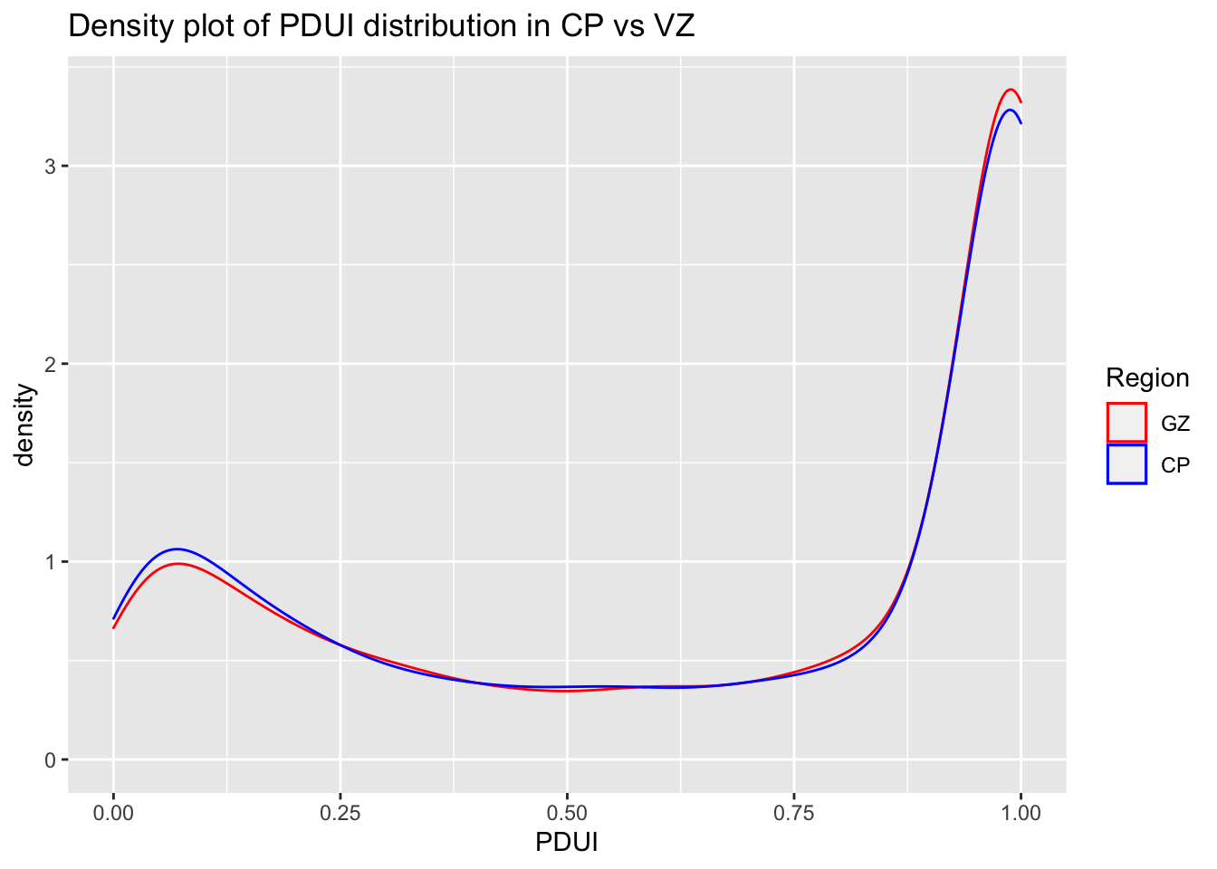
#Density plot of PDUI distribution in CP vs VZ
ggplot(data = PDUIS.averaged.stats) +
  geom_density(mapping = aes(x = CP.PDUI, color = "red")) +
  geom_density(mapping = aes(x = VZ.PDUI, color = "blue")) +
  scale_color_manual(name = "Region", values = c('red' = 'red', 'blue' = 'blue'), labels = c('GZ', 'CP')) +
  labs(title = "Density plot of PDUI distribution in CP vs VZ", x = "PDUI")

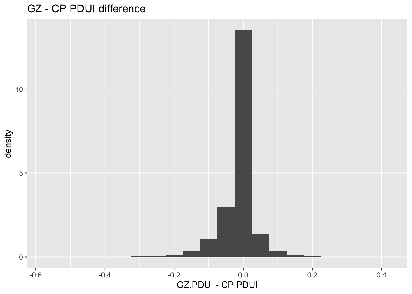
#Histogram of distributions of VZ - CP difference
ggplot(data = PDUIS.averaged.stats) +
  geom_histogram(mapping = aes(x = vz.cp.diff, y = after_stat(density)), binwidth = 0.05) +
  labs(title = "GZ - CP PDUI difference", x = "GZ.PDUI - CP.PDUI")

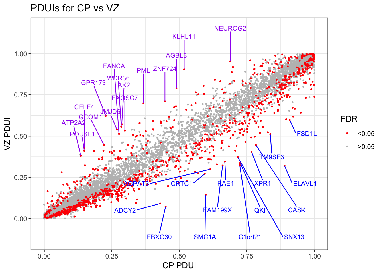
Plot CP vs VZ PDUI, denote transcripts with significant difference (FDR < 0.05 as per repeat measures ANOVA)

#Get transcripts with significantly different PDUIs based on FDR cutoff of 0.05, separate to increased or decreased PDUI in CP compared to VZ. 
vz.cp.neg.sig =  PDUIS.averaged.stats %>% filter(FDR < 0.05, vz.cp.diff < 0)
vz.cp.pos.sig = PDUIS.averaged.stats %>% filter(FDR < 0.05, vz.cp.diff > 0)
vz.cp.neg.sig <- arrange(vz.cp.neg.sig, by = FDR)
vz.cp.pos.sig = arrange(vz.cp.pos.sig, by = FDR)

#Get top 10 genes from vz.cp.neg.sig and vz.cp.pos.sig
vz.cp.pos.sig <- vz.cp.pos.sig %>% arrange(-vz.cp.diff)
vz.cp.neg.sig <- vz.cp.neg.sig %>% arrange(vz.cp.diff)

neg.sig.top10 <- vz.cp.neg.sig[1:15,]
pos.sig.top10 <- vz.cp.pos.sig[1:15,]


Fig3D=ggplot(data = PDUIS.averaged.stats) +
  geom_point(mapping = aes(x = CP.PDUI, y = VZ.PDUI, color = cut(FDR, c(0, 0.05, Inf))), size = 0.5) +
  scale_color_manual(values=c("red", "gray"), labels = c("<0.05", ">0.05")) +
  labs(title = "PDUIs for CP vs VZ", x = "CP PDUI", y = "VZ PDUI", color = "FDR") +
  geom_text_repel(data = neg.sig.top10, mapping = aes(x = CP.PDUI, y = VZ.PDUI, label = geneNames), color = "blue", min.segment.length = 0, box.padding = 1, max.overlaps = Inf, size=3,force = 20, nudge_y = -.2) +
  geom_text_repel(data = pos.sig.top10, mapping = aes(x = CP.PDUI, y = VZ.PDUI, label = geneNames), color = "purple", min.segment.length = 0, box.padding = 0, max.overlaps = Inf, size=3,force = 20, nudge_y = .2) + theme_bw()

Fig3D

ggsave(file='output/figures/Fig3/Fig3D_APA.pdf', width=5,height=4)

Pathway enrichment of top transcript PDUI changes using gprofiler2.

library(gprofiler2)

#Order significant genes by descending vz.cp.diff
vz.cp.neg.sig <- vz.cp.neg.sig %>% arrange(vz.cp.diff) ## Ordered by effect size
vz.cp.pos.sig <- vz.cp.pos.sig %>% arrange(-vz.cp.diff) ## Ordered by effect size
all.sig <- rbind(vz.cp.neg.sig, vz.cp.pos.sig)
all.sig <- all.sig %>% arrange(-abs(vz.cp.diff))

gostres.neg <- gost(query = vz.cp.neg.sig$geneNames, organism = "hsapiens", ordered_query = FALSE, significant = TRUE, custom_bg = PDUIS.averaged.stats$geneNames, correction_method = "fdr",sources = c("GO", "KEGG", "REAC"))

Detected custom background input, domain scope is set to 'custom'

as_tibble(gostres.neg$result)

# A tibble: 64 × 14
   query   signi…¹ p_value term_…² query…³ inter…⁴ preci…⁵ recall term_id source
   <chr>   <lgl>     <dbl>   <int>   <int>   <int>   <dbl>  <dbl> <chr>   <chr> 
 1 query_1 TRUE    3.00e-5    5445     653     510  0.781  0.0937 GO:000… GO:CC 
 2 query_1 TRUE    1.59e-4    2462     653     259  0.397  0.105  GO:004… GO:CC 
 3 query_1 TRUE    1.59e-4    2462     653     259  0.397  0.105  GO:004… GO:CC 
 4 query_1 TRUE    1.59e-4    2775     653     287  0.440  0.103  GO:003… GO:CC 
 5 query_1 TRUE    1.59e-4      59     653      18  0.0276 0.305  GO:001… GO:CC 
 6 query_1 TRUE    5.03e-4    2522     653     261  0.400  0.103  GO:003… GO:CC 
 7 query_1 TRUE    4.07e-3    2998     653     294  0.450  0.0981 GO:007… GO:CC 
 8 query_1 TRUE    4.07e-3     163     653      29  0.0444 0.178  GO:003… GO:CC 
 9 query_1 TRUE    4.07e-3    2998     653     294  0.450  0.0981 GO:003… GO:CC 
10 query_1 TRUE    4.07e-3    2998     653     294  0.450  0.0981 GO:004… GO:CC 
# … with 54 more rows, 4 more variables: term_name <chr>,
#   effective_domain_size <int>, source_order <int>, parents <list>, and
#   abbreviated variable names ¹significant, ²term_size, ³query_size,
#   ⁴intersection_size, ⁵precision

gostres.pos <- gost(query = vz.cp.pos.sig$geneNames, organism = "hsapiens", ordered_query = FALSE, significant = TRUE, custom_bg = PDUIS.averaged.stats$geneNames, correction_method = "fdr", 
                    sources = c("GO", "KEGG", "REAC"))

Detected custom background input, domain scope is set to 'custom'

No results to show
Please make sure that the organism is correct or set significant = FALSE

# No significant pathway enrichments from genes with significantly longer PDUI in VZ vs CP

gostres_all <- gost(query = all.sig$geneNames, organism = "hsapiens", ordered_query = FALSE, significant = TRUE, custom_bg = PDUIS.averaged.stats$geneNames, correction_method = "fdr", sources = c("GO", "KEGG", "REAC"))

Detected custom background input, domain scope is set to 'custom'

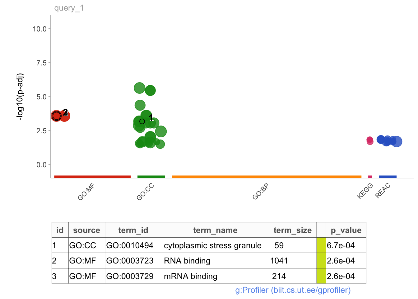
# No significant pathway enrichments when genes are ranked in order of decreasing magnitude of PDUI change between brain regions

#Working with all significant genes:
gostplot(gostres_all, capped = FALSE, interactive = T)

gostres_out <- subset(gostres_all$result, select = c("significant", "p_value", "term_size", "query_size", "intersection_size", "precision", "recall", "term_id", "source", "term_name", "effective_domain_size", "source_order"))
write.table(gostres_out, "output/tables/TableS3_APA_GO_results.txt")

#GO plot with RNA binding terms highlighted
rna_terms <- c("RNA binding", "mRNA binding", "cytoplasmic stress granule")
rna_gostres_all <- subset(gostres_all$result, term_name %in% rna_terms)
publish_gostplot(gostplot(gostres_all, capped = FALSE, interactive = FALSE), highlight_terms = rna_gostres_all$term_id)

Overrepresentation analysis: are transcripts w/significantly different PDUIs enriched for RBPs & TFs compared to background genes? Use RBP list from Gebauer et al. 2021

#Load RBP gene list from Gebauer et al. 2021
RBPs <- scan("ref/RBPs/rbps_gebauer_nrg_2021.txt", what = "", sep = "\n")

#Get background genes (transcripts with no significant change in PDUI)
PDUIS.averaged.bckgrd <- PDUIS.averaged.stats %>% filter(FDR >= 0.05)

bckgrd.rbp <- nrow(subset(PDUIS.averaged.bckgrd, geneNames %in% RBPs))
bckgrd.nonrbp <- nrow(subset(PDUIS.averaged.bckgrd, !geneNames %in% RBPs))

sig.rbp <- nrow(subset(PDUIS.averaged.stats %>% filter(FDR < 0.05), geneNames %in% RBPs))
sig.nonrbp <- nrow(subset(PDUIS.averaged.stats %>% filter(FDR < 0.05), !geneNames %in% RBPs))

#Run one-sided Fisher's exact test
d <- data.frame(bckgrd = c(bckgrd.rbp, bckgrd.nonrbp), sig = c(sig.rbp, sig.nonrbp))
row.names(d) <- c("RBP", "non-RBP")

d

        bckgrd sig
RBP       3074 453
non-RBP   5809 560

fisher.test(d, alternative = "less")


    Fisher's Exact Test for Count Data

data:  d
p-value = 2.06e-10
alternative hypothesis: true odds ratio is less than 1
95 percent confidence interval:
 0.0000000 0.7321337
sample estimates:
odds ratio 
 0.6541755