Rows: 214516 Columns: 35
── Column specification ────────────────────────────────────────────────────────
Delimiter: "\t"
chr  (7): annot_gene_id, annot_transcript_id, annot_gene_name, annot_transcr...
dbl (28): gene_ID, transcript_ID, n_exons, length, 209_1_VZ, 209_2_VZ, 209_3...

ℹ Use `spec()` to retrieve the full column specification for this data.
ℹ Specify the column types or set `show_col_types = FALSE` to quiet this message.
Warning in bicor(datExpr, datME, , use = "p"): bicor: zero MAD in variable 'x'.
Pearson correlation was used for individual columns with zero (or missing) MAD.
Warning: One or more parsing issues, see `problems()` for details
Rows: 18321 Columns: 26
── Column specification ────────────────────────────────────────────────────────
Delimiter: "\t"
chr  (8): gene_id, group, OR (PTV), OR (Class I), OR (Class II), OR (PTV) up...
dbl (16): Case PTV, Ctrl PTV, Case mis3, Ctrl mis3, Case mis2, Ctrl mis2, P ...
lgl  (2): De novo mis3, De novo mis2

ℹ Use `spec()` to retrieve the full column specification for this data.
ℹ Specify the column types or set `show_col_types = FALSE` to quiet this message.
Rows: 119958 Columns: 20
── Column specification ────────────────────────────────────────────────────────
Delimiter: "\t"
chr  (4): gene_id, group, damaging_missense_fisher_gnom_non_psych_OR, ptv_fi...
dbl (16): n_cases, n_controls, damaging_missense_case_count, damaging_missen...

ℹ Use `spec()` to retrieve the full column specification for this data.
ℹ Specify the column types or set `show_col_types = FALSE` to quiet this message.
Rows: 71456 Columns: 12
── Column specification ────────────────────────────────────────────────────────
Delimiter: "\t"
chr (2): gene_id, group
dbl (9): xcase_lof, xctrl_lof, pval_lof, xcase_mpc, xctrl_mpc, pval_mpc, xca...
lgl (1): pval_infrIndel

ℹ Use `spec()` to retrieve the full column specification for this data.
ℹ Specify the column types or set `show_col_types = FALSE` to quiet this message.
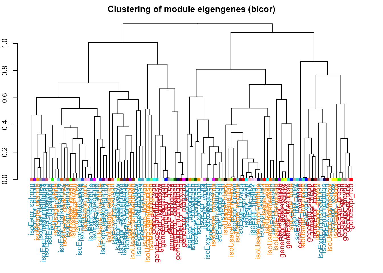
df1 =data.frame(net.isoFr$MEs$eigengenes)colnames(df1) =paste0("isoUsage_", gsub("ME", "", colnames(df1)))df2 =data.frame(net.isoExpr$MEs$eigengenes)colnames(df2) =paste0("isoExpr_", gsub("ME", "", colnames(df2)))df3 =data.frame(net.geneExpr$MEs$eigengenes)colnames(df3) =paste0("geneExpr_", gsub("ME", "", colnames(df3)))df =cbind(df1,df2,df3)tree =hclust(as.dist(1-bicor(df)),method ='average')# Hierarchically cluster the sample-eigenegene correlations# and save the dendrogram representationdist_mat <-as.dist(1-bicor((df)))clust <-hclust(dist_mat,method ='average')dend <-as.dendrogram(clust)# Define the mapping between network names and colorslabelColors =list("geneExpr"="#d62828","isoExpr"="#219ebc","isoUsage"="#ff9914")# Iterate over the dendrogram leafs and manually change the node# parameters according to the label name (the column name)colLab <-function(n) {if (is.leaf(n)) {# Grab the attributes of the leaf/node a <-attributes(n)# Print the name so that later on you can arrange the heatmap# to match the order in the dendrogramcat(as.character(a$label))cat(", ")# Extract the name of the network (this regex extracts dev_gene from dev_gene_blahblah) net_name <-str_extract(a$label, "[:alnum:]+")# Assign the text color according to the mapping in labelColorsif (net_name %in%names(labelColors)) { labCol <- labelColors[[net_name]] } else { labCol <-"#5603ad" }# Assign the node color to match the WGCNA color (saddlebrown, turquoise, etc.) mod_color <-str_match(a$label,"[^_]+_(.*)")[2]# Add the new node attributes onto the existing node attributesattr(n, "nodePar") <-list(a$nodePar,cex =1,pch =15,lab.col = labCol, # This is the color of the leaf label (the text)col = mod_color) # This is the color of the leaf (the square) }return(n)}# Apply the iteration function onto our saved dendrogramnew_dendro <-dendrapply(dend, colLab)
# Plot the resulting dendrogramoptions(repr.plot.width =30, repr.plot.height =5, repr.plot.res =600)par(cex=0.8, mar =c(10,2,2,2))plot(new_dendro,main ="Clustering of module eigengenes (bicor)",xlab ="", sub ="")
Warning in bicor(datExpr, datME, , use = "p"): bicor: zero MAD in variable 'x'.
Pearson correlation was used for individual columns with zero (or missing) MAD.
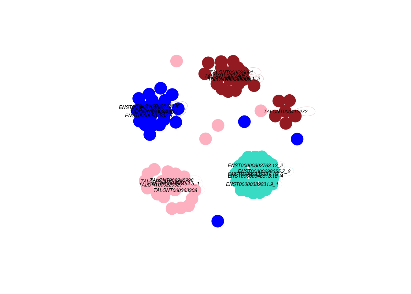
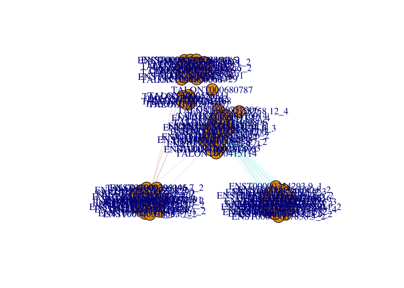
isoTOM =TOMsimilarityFromExpr(t(this_datExpr[hubs25,]),networkType ='signed', power =14)
TOM calculation: adjacency..
..will not use multithreading.
 Fraction of slow calculations: 0.000000
..connectivity..
..matrix multiplication (system BLAS)..
..normalization..
..done.
isoTOM =TOMsimilarityFromExpr(t(this_datExpr[hubs25,]),networkType ='signed', power =14)
TOM calculation: adjacency..
..will not use multithreading.
 Fraction of slow calculations: 0.000000
..connectivity..
..matrix multiplication (system BLAS)..
..normalization..
..done.